Part 1: Image Classification
In this section, I have trained a convolutional neural network to classify the
Fashion MNIST dataset into 10 different classes: top, trouser, pullover, dress,
coat, sandal, shirt, sneaker, bag, and ankle-boot.
1.1 CNN Architecture
My CNN consists of 2 convolution layers with 32 channels each. Each convolution
layer is followed by a ReLU nonlinearity and 2x2 maxpooling layer. It is then
followed by 2 fully connected networks with a ReLU applied after the first fully
connected layer. I trained this network using the Adam optimizer over 15 epochs
with a learning rate of 1e-3, a weight decay of 1e-5, and batch size 40.
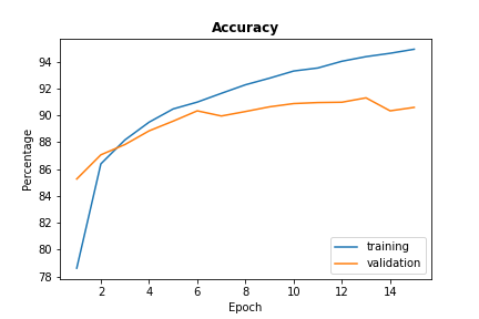
1.2 Model Accuracy
The plot below shows how the network improves over time. By the 8th epoch, the learning
has pretty much converged while the accuracy of the training set shows increased improvement,
suggesting overfitting on the training set.
1.3 Class Accuracy
The chart below shows the results of the CNN tested on the validation set and the test set.
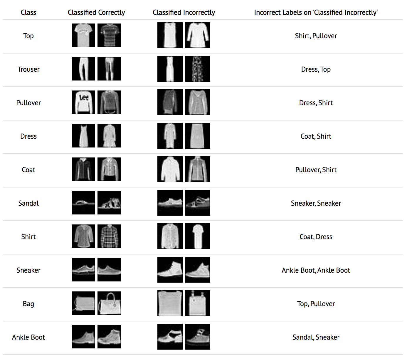
As you can see, the CNN does the worst job at classifying a shirt, probably because there's
more variation in shape and style of the shirts compared to the other classes. The overall
accuracy of both the validation and test sets is 90%.
| Class |
Test Accuracy |
Val Accuracy |
| Top |
82% |
84% |
| Trouser |
98% |
99% |
| Pullover |
91% |
91% |
| Dress |
85% |
87% |
| Coat |
84% |
82% |
| Sandal |
97% |
97% |
| Shirt |
72% |
73% |
| Sneaker |
93% |
94% |
| Bag |
97% |
97% |
| Ankle Boot |
97% |
98% |
Here we have some examples of images that were classified either correctly or
incorrectly by the network.
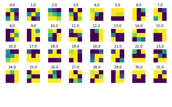
1.3 Visualizing the Learned Filters
These are the 32 filters learned by the first convolution layer:
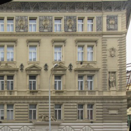
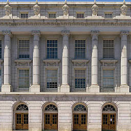
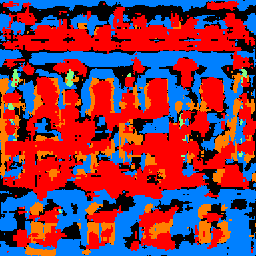
Part 2: Semanatic Segmentation
This section looks at the Mini Facade dataset and aims to train a network
that is able to accurately convert a given image into its semantic segmentation label. The dataset
consists of a variety of images of buildings across the world so we can train our network to
recognize the 5 different classes (other, facade, pillar, window, and balcony) and assign it the correct
pixel color.
2.1 CNN Architecture
My model has 6 convolution layers with 64, 64, 128, 128, 256, and 5 channels respectively, all with a kernel size 3 and padding of 1.
There are also two ConvTranspose layers each with kernel size 2 and stride 2 at the end to handle upsampling.
The structure is as follows:
1. conv2d(64 channels) → ReLU
2. conv2d(64 channels) → ReLU → 2x2 MaxPool2d
3. conv2d(128 channels) → ReLU
4. conv2d(128 channels) → ReLU → 2x2 MaxPool2d
5. convTranspose2d(128 channels) → conv2d(256 channels)
6. convTranspose2d(256 channels) → conv2d(5 channels)
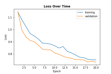
To train the model, I use the Adam optimizer with a learning rate of 1e-3 and weight decay of 1e-5.
I trained the model over 20 epochs with a batch size of 5. Below is a graph displaying the loss over time
on the training and validation sets.
2.2 Results: Average Precision
The average precision on my test set came down to 0.58. Each class AP is shown below.
AP = 0.6627658634014512 (Other)
AP = 0.7748032505153853 (Facade)
AP = 0.1436585109758356 (Pillar)
AP = 0.8230532488307044 (Window)
AP = 0.5039691926403682 (Balcony)
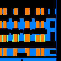
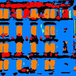
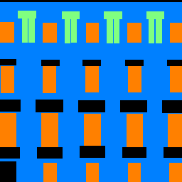
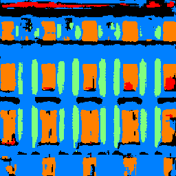
Some results on the test images:
| Image |
Ground Truth |
Model Prediction |
|
|
|
|
|
|
|
|
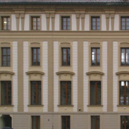
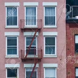
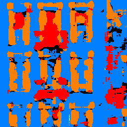
And here are some results on my own images:
The network does a pretty good job identifying windows and facades on the test set
as evidenced by having the highest APs. With the lowest AP of 0.14, the pillars were
definitely the most variable in each output. On my own inputs, you can see the similar
consistency in identifying windows and facades. However, there's some variability in Wheeler Hall's windows
because some have its blinds shut while some are partially open or fully open. The network
doesn't seem to be familiar with "different types of window" situations and therefore incorrectly
identified some parts as balconys. Similarly with the test set, the pillars are the hardest
to identify.