|
|
This project contains two parts: a. image classification b. semantic segementatio.
In both parts, I am using deep neural network to solve the problem.
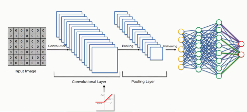
For image classification, I run the training data through the network, which composes of convolutional layers and fully connected layers, calculate the loss and try to optimize the loss through back propagation. By continuously updating the weights, I am able to arrive at the relatively good set of parameters for the desired classification. Then, I tested the trained network on the test data to see how the network perform when given new data.
For semantic segmentation, the procedure is pretty much the same, except for the fact that the network composes of convolutional layers only in order to match the input size and the output size. Yet convolutional layers inevitably reduces the size of the image, as a result, I used transpose convolution layers to upscale the image size.
Definition: The number of training examples used in the estimate of the error gradient is a hyperparameter for the learning algorithm called the “batch size,” or simply the “batch.”
The larger the batch, the more accurate the update of the parameters will be in the gradient descent. Two extreme cases will be 1) passing one image per batch 2) passing all images as a batch. In the first case, the inputs are noisy, which can be a regularization effect to prevent overgeneralization. In the second, the gradient descent will learn better but there might be overgeneralization based on the input data. Finally, it also relates to the speed and stability of the learning process. I
Definition: In gradient descent, the model finds the global minimum through continously making small "leaps" in the direction of the gradient. The length of the step is determined by the learning rate.
Generally, a large learning rate allows the model to learn faster, at the cost of arriving on a sub-optimal final set of weights. A smaller learning rate may allow the model to learn a more optimal or even globally optimal set of weights but may take significantly longer to train.
In general, large weights will cause over-generalization. By adding an L2 regularization of the weight, the model can prevent overfitting.
 Here is a list of common optimizers in Pytorch that I will try for my model.

		torch.optim.Adadelta(params, lr=1.0, rho=0.9, eps=1e-06, weight_decay=0)
 torch.optim.Adagrad(params, lr=0.01, lr_decay=0, weight_decay=0, initial_accumulator_value=0, eps=1e-10)
 torch.optim.Adam(params, lr=0.001, betas=(0.9, 0.999), eps=1e-08, weight_decay=0, amsgrad=False)
 torch.optim.SGD(params, lr=0.01, momentum=0/9, dampening=0, weight_decay=0.01, nesterov=False)
|
        self.conv1 = nn.Conv2d(1, 32, 3)


        x = F.relu(x)


        x = F.max_pool2d(x, 2, stride = 2)


        self.conv2 = nn.Conv2d(32, 32, 3)


        x = F.relu(x)


        x = F.max_pool2d(x, 3)


        self.fc1 = nn.Linear(288, 120)


        self.fc2 = nn.Linear(120, 10)


        x = F.relu(x)
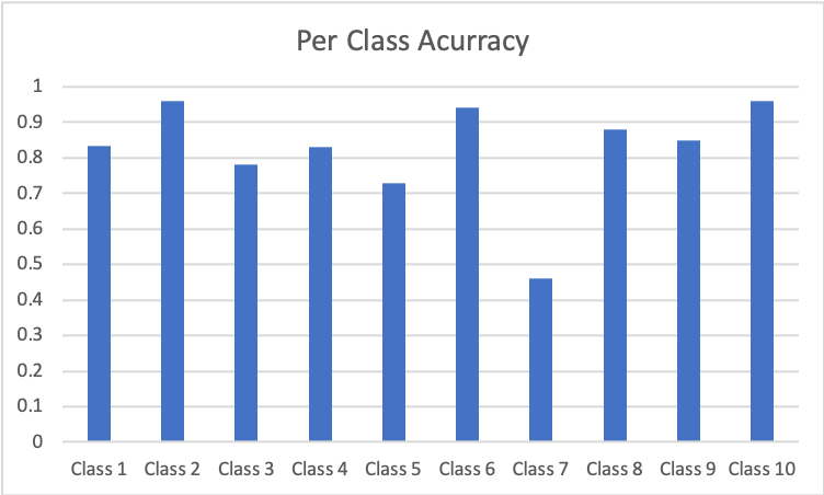
In general, the accuracy of classification increases as the network iterate through the data. This following image is based on the model with architecture above and parameters: a. Batch size 20 b. Learning rate 0.01 c. Weigh Decay 0.
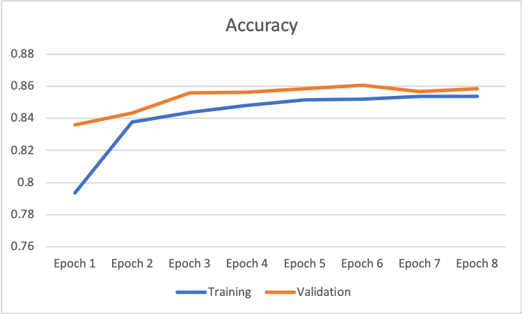 |
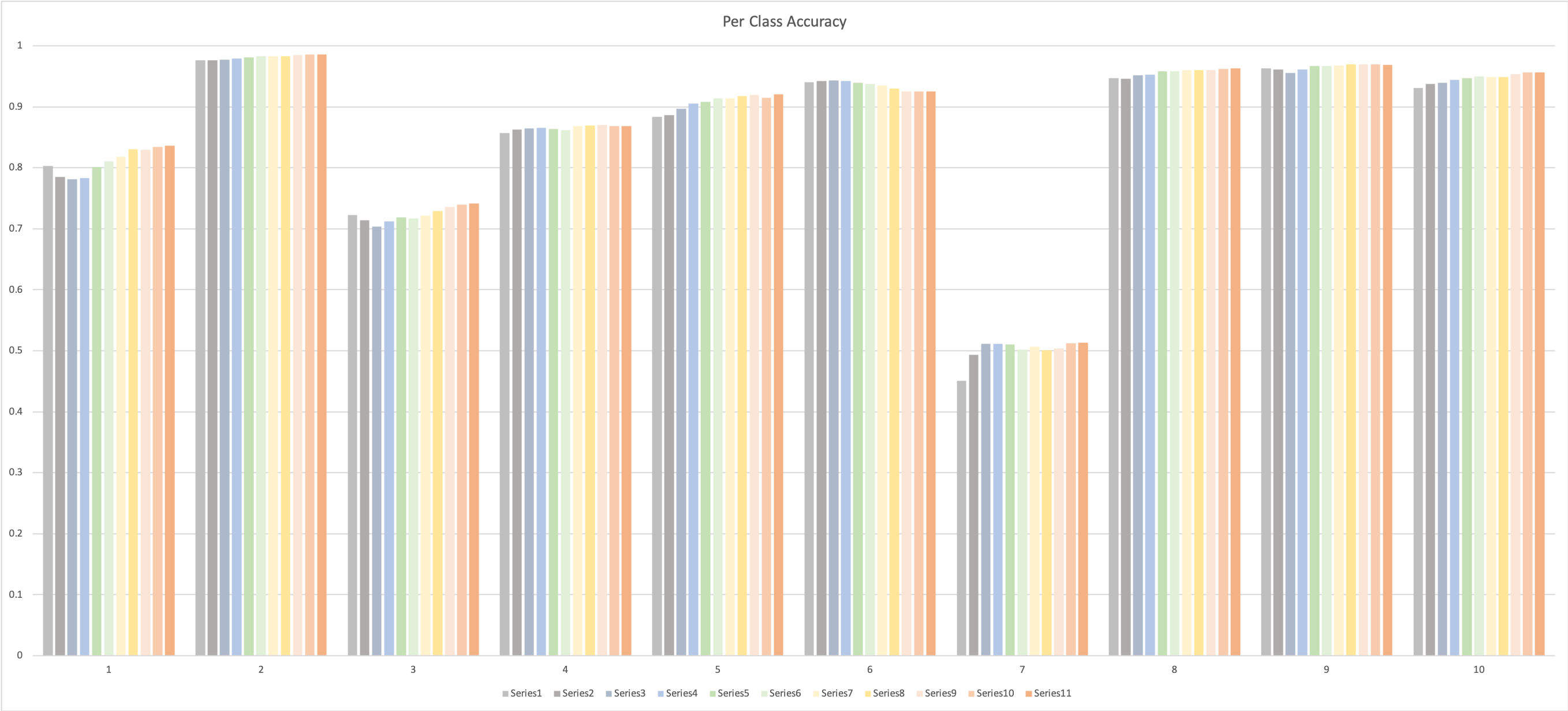
Then, I went on to fine tune the network within the current architecture in order to get the best classification performance. I first tried to increase the batch size. Then, I decreased the learning rate and added the L2 regularization for the weights. In the end, I tried different optimizer. I managed to increase the accuracy from 83% to 87%.
Parameters: a. Batch size 256 b. Learning rate 0.001 c. Weigh Decay 0.001 |
|
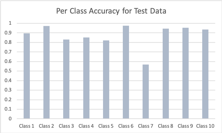
Parameters: a. Batch size 20 b. Learning rate 0.01 c. Weigh Decay 0 |
|
 |
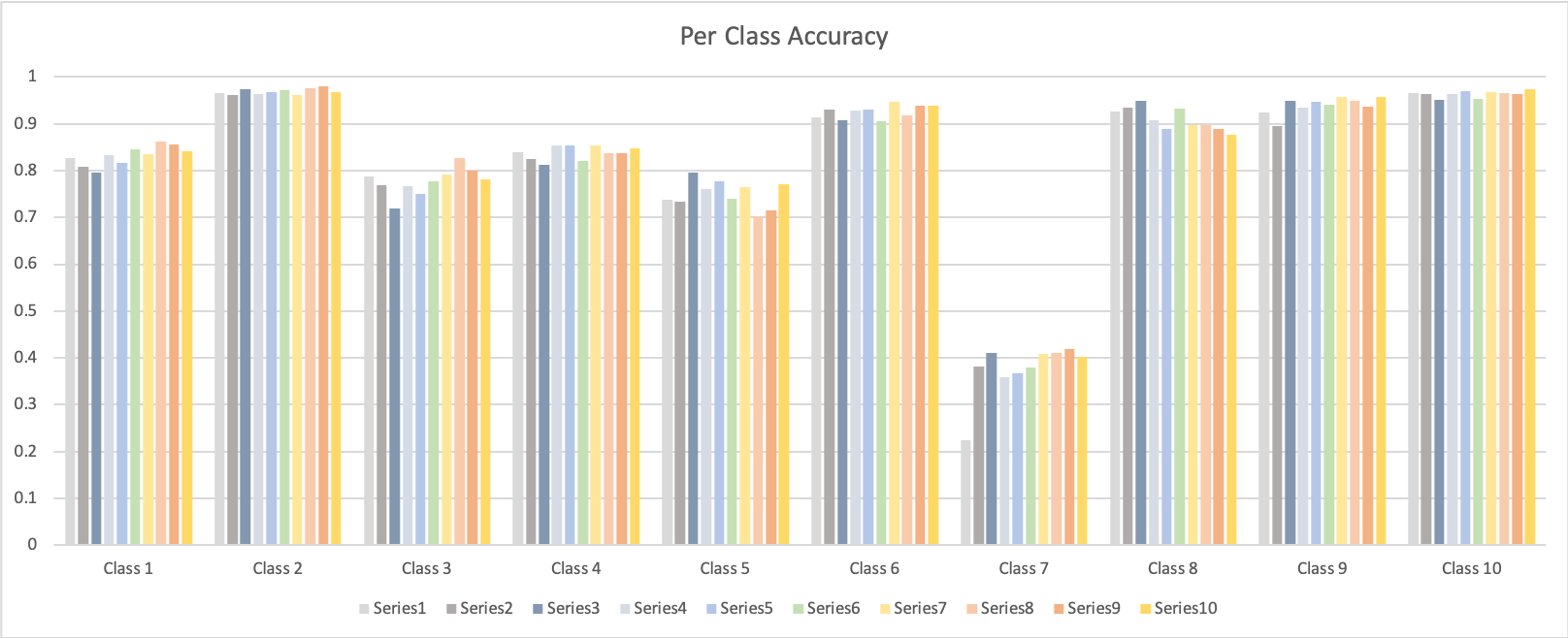 |
In both networks, Class 7 is the hardest to get, while Class2 and Class 10 is the easiest to get.
Then I changed the optimizer to SGD to see the results. By Running on the test data, I get a loss of 0.5055486790835857 and accuracy of 8160/10000 with class accuracy of
[0.72821577 0.953125 0.72897196 0.91073124 0.75460123 0.85813492 0.41444867 0.93793794 0.93698347 0.94651867]
which is worse than using Adam.
Then I moved on to fine tune the architecture. Since I can change the filter size, the stride, the padding and the neuron number of the fully connected network. The results are not as good as the current architecture.
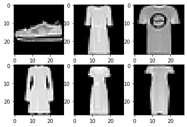
The following shows the correctly classified images from class 0 to class 9.
 |
 |
 |
 |
 |
 |
 |
 |
 |
 |
 |
 |
 |
 |
 |
 |
 |
 |
 |
 |
The following shows the incorrectly classified images from class 0 to class 9.
 |
 |
 |
 |
 |
 |
 |
 |
 |
 |
 |
 |
 |
 |
 |
 |
 |
 |
 |
 |
 |
 |
 |
 |
 |
 |
 |
 |
 |
 |
 |
 |
 |
 |
 |
 |
 |
 |
 |
 |
 |
 |
 |
 |
 |
 |
 |
 |
 |
 |
 |
 |
self.n_class = N_CLASS
self.conv1 = nn.Conv2d(3, 64, 3)
self.conv2 = nn.Conv2d(64, 128, 3)
self.conv3 = nn.Conv2d(128, 256, 3)
self.deconv1 = nn.ConvTranspose2d(256, 128, 3)
self.deconv2 = nn.ConvTranspose2d(128, 64, 3)
self.deconv3 = nn.ConvTranspose2d(64, 5, 3)
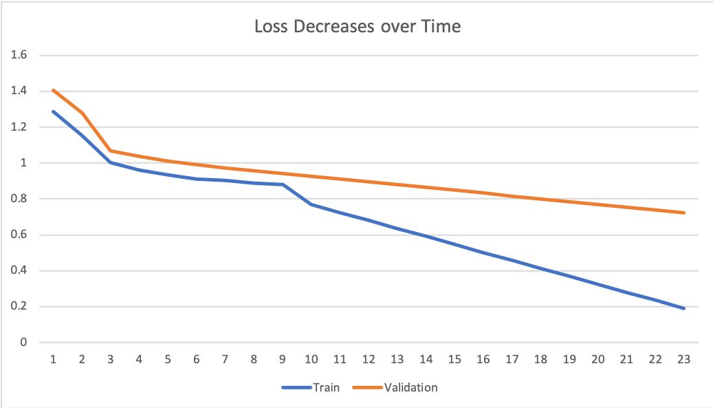
batch_size = 8
epoch = 23
criterion = nn.CrossEntropyLoss()
optimizer = torch.optim.Adam(net.parameters(), 1e-3, weight_decay=1e-5)
 |
| Black | Blue | Green | Orange | Red | Average |
| 0.5459 | 0.6559 | 0.0264 | 0.6666 | 0.5480 | 0.482 |
My network did a good job on segmenting the window, the panel and the wall. It did poorly on identifying the pillar and the balcony. This may due to the lack of sufficient information in the training set on pillar and balcony.
 |
 |