Classification and Segmentation
Jingwei Kang, cs194-26-abr
Overview
Part 1: Image Classification
Network Details
In this part of the project, I learned to create a convolutional neural network to classify different articles of clothing in the Fashion-MNIST dataset. The network had two convolutional layers with 32 channels of size 3 kernels, each followed by a ReLU and max pooling layer. These convolutional layers are followed by two fully connected layers, with a ReLU after the first fully connected layer. The last fully connected layer has 10 output nodes, each representing the probabilities for the 10 classes in the dataset. I initially used a learning rate of 0.01 with the Adam optimizer, but reduced the learning rate to 0.001 after noticing the loss oscillating without improving. I trained the model to convergence (loss in successive calculations was less than 0.0001). This translated to increasing the number of epochs from 2 to 10.
Results
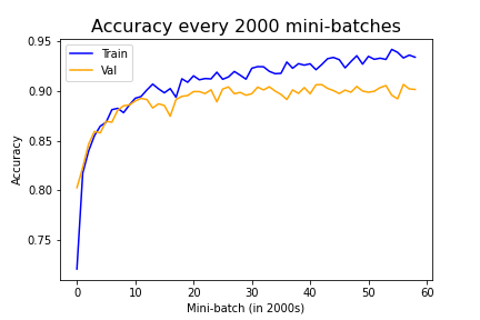
Accuracy Over Training Process
Prior to training, we split the training data into a training and validation set (for tuning our hyperparameters). We can visualize the accuracy for each over the training process below. Note that at around the 10th mini-batch (around the 2nd epoch), we do notice the training accuracy diverge from the validation accuracy, suggesting we may be starting to overfit.
|
Per Class Accuracy
Below we show the accuracy for each class of image, as well as some examples of images that were correctly and incorrectly classified. In total, our average validation and test accuracy were both 90%.
| Class (#) | Colloquial | Validation Acc. | Test Acc. | Sample Images |
|---|---|---|---|---|
| 0 | T-shirt/top | 83% | 84% | 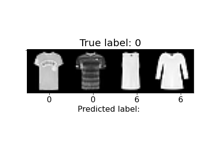 |
| 1 | Trouser | 98% | 98% | 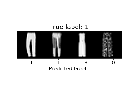 |
| 2 | Pullover | 88% | 85% | 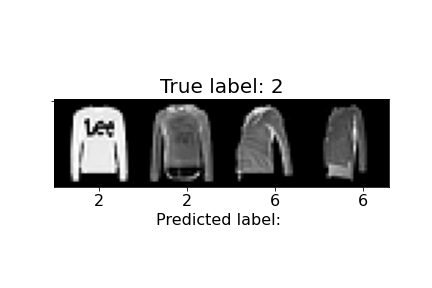 |
| 3 | Dress | 87% | 87% | 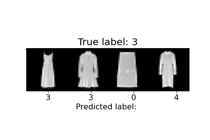 |
| 4 | Coat | 80% | 82% | 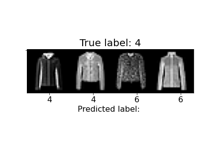 |
| 5 | Sandal | 97% | 97% | 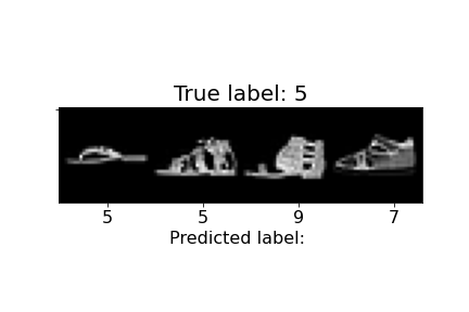 |
| 6 | Shirt | 74% | 73% | 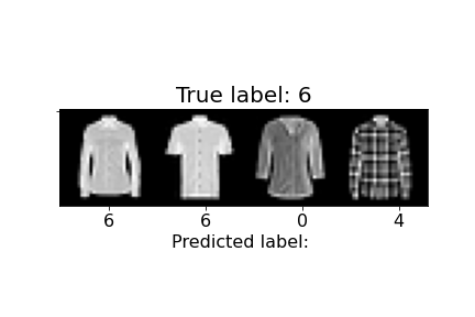 |
| 7 | Sneaker | 97% | 98% | 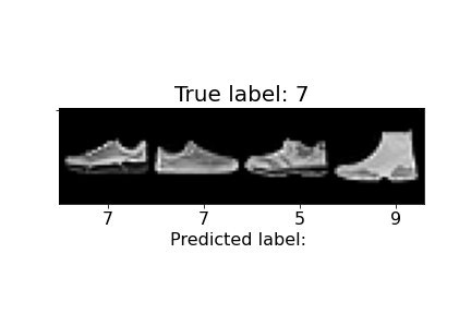 |
| 8 | Bag | 98% | 97% | 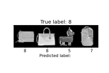 |
| 9 | Ankle boot | 93% | 93% | 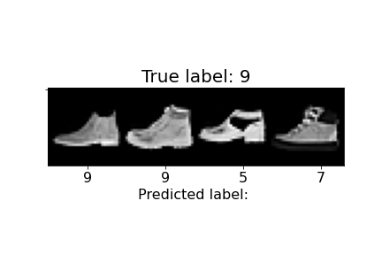 |
Above, we can observe how some of the misclassifications occurred. For example, the last sandal was misclassified as a sneaker. We can notice the higher ankle support and a heel present in the sandal, similar to the sneakers. The second to last sandal was misclassified as an ankle boot and we see similar characteristics, but with an even higher ankle. In general, shirts and coats were the hardest to classify, probably due to variations in length, color, and design.
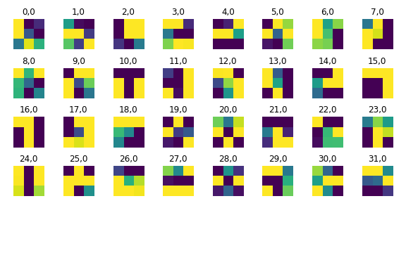
Filter Visualization
The 32 filters from the first convolutional layer (1 channel input, 32 channel output) are shown below.
|
Part 2: Semantic Segmentation
Network Details
In this part, I aimed to identify each pixel in an image with the correct architechtural class (facade, pillar, window, balcony, others). The network was designed to increase the number of channels as I moved from a higher resolution image to a lower resolution one (through max pooling), and decrease the number of channels as I moved from lower resolution to higher resolution (through upsampling/transposed convolution). There were no fully connected layers - in fact, the last convolutional layer had the same dimensions as the original image, with 5 total channels (1 for each architectural class). This allows us to classify each individual pixel rather than the whole image (in Part 1). The layers used in my network are listed below. Any parameters not listed use the default values in Pytorch.
- Conv2d(in_channels=3, out_channels=32, kernel_size=3, padding=1)
- ReLU()
- MaxPool2d(kernel_size=2)
- Conv2d(in_channels=32, out_channels=64, kernel_size=3, padding=1)
- ReLU()
- ConvTranspose2d(in_channels=64, out_channels=32, kernel_size=3, stride=2, padding=0)
- Conv2d(in_channels=32, out_channels=5, kernel_size=2, padding=0)
Results
Loss Over Training Process
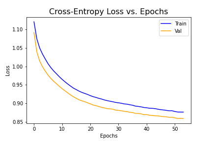
As we can see below, the cross-entropy loss decreased for both the training and validation sets over the 30 epochs. Oddly enough, the validation loss was lower than the training loss. I would expect the training losses to be lower because that is what the model is training on, and this is actually the case when I use the dummy model initially provided to us. This happened despite running to convergence such that subsequent losses differ by less than 0.0001. It could be due to the way I split the training data into the training and validation sets. The dataloader written for us didn't seem to allow a simple function call to randomly split the data (as with Part 1), so I specified the first 800 images to be the training set and the last 106 images to be the validation set. The other discrepancy was the batch size (I used 4 for the train and 1 for the validation), but it seems like the losses were normalized for the number of samples. Ultimately, I wasn't able to reconcile this discrepancy but was able to still generate decent results.
|
Average Precision
| Pixel Value | Color | Class | Test AP |
|---|---|---|---|
| 0 | black | others | 0.654 |
| 1 | blue | facade | 0.738 |
| 2 | green | pillar | 0.109 |
| 3 | orange | window | 0.727 |
| 4 | red | balcony | 0.307 |
| - | - | Overall | 0.507 |
As we see above, pillars and balconies are the most difficult to classify, possibly because they have lower representation in the datasets.
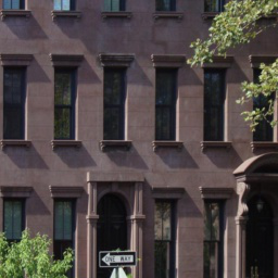
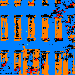
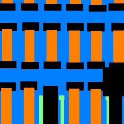
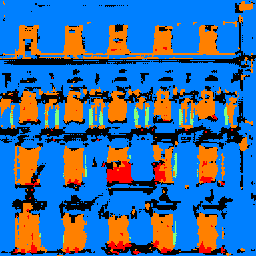
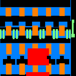
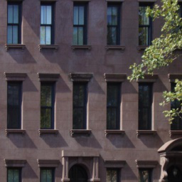
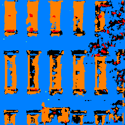
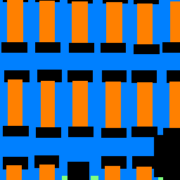
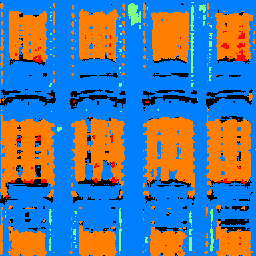
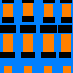
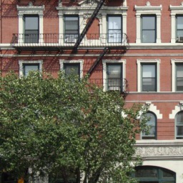
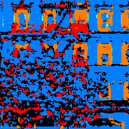
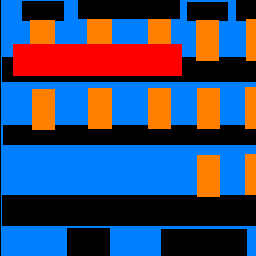
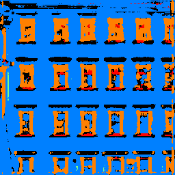
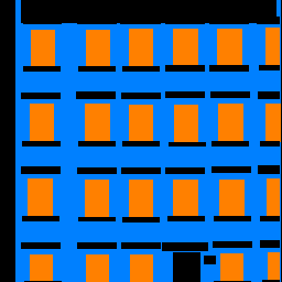
Sample Images
The sample images below support the idea that we simply don't have as many pillars and balconies present in images.
| Original | Predicted Labels | Ground Truth |
|---|---|---|
 |
 |
 |
 |
 |
 |
 |
 |
 |
 |
 |
 |
 |
 |
 |
 |
 |
 |