Part 1: Image Classification
Objective
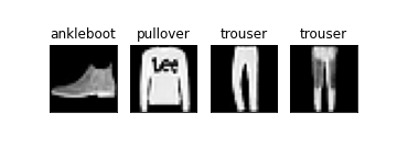
Fashion MNIST is a dataset of 60,000 training images and 10,000 test images about ten different classes of apparel and accessories. It is designed as a direct drop-in to its bigger brother, MNIST. In this section, we use convolutional neural nets (CNN) to classify images such as the ones below.
Network Layout
I followed the layout given in the spec for the CNN architecture. It consists of 2 convolution layers, and 2 fully connected affine layers. Both convolution layers contain 32 output filters. The first affine layer has an output size of 100, while the second has an output of 10 to match the number of classes in the dataset.
[conv(32) - relu - maxpool(2)] x 2 - affine(100) - relu - affine(10) The convolution layers used a square filter of length 7. For the first layer, I added padding such that the output image size stays the same as the input; though I admit this was somewhat arbitrary.
Training Procedure
I downloaded the Fashion MNIST training dataset and randomly separated it to a training set of 50k images and a validation set of 10k. I used a batch size of 32 and a learning rate of 0.01 to train my network by minimizing cross-entropy loss for 20 epochs.
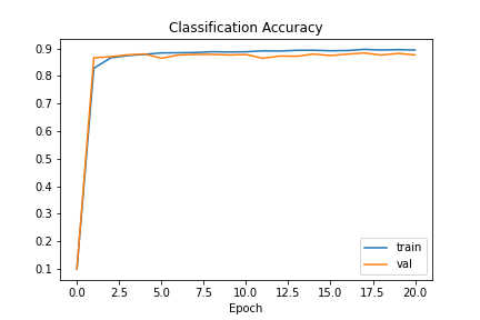
Afterwards, I did some experimentation by further training the network with smaller and smaller learning rates. The theory is that the smaller rate (I went down to 0.003) allows better fine-tuning of parameters to hit the extra percentage point or two.
Evaluating Performance
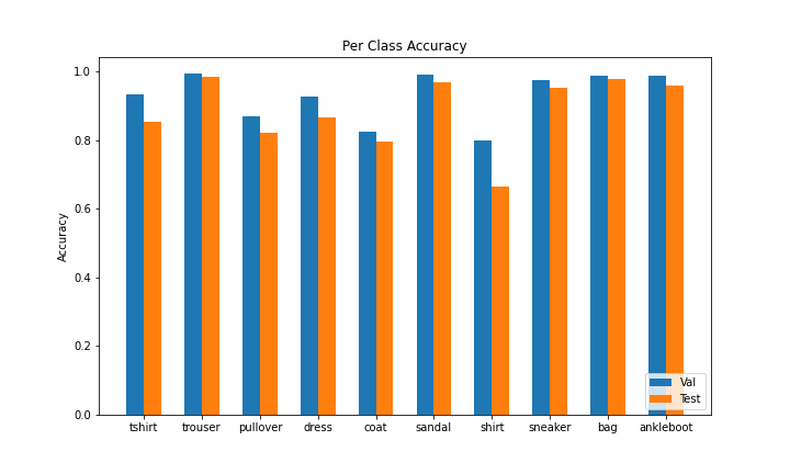
When ran on the Fashion MNIST test dataset of 10k images, my final CNN achieved a respectable classification accuracy of 88.5%. When further analyzing the per-class accuracy, I found that the network performed the worst on "shirt", "coat", and "pullover", which is understandable given how similar these clothing articles are.
| Class | Val Accuracy | Test Accuracy |
|---|---|---|
| T-shirt/top | 0.932 | 0.855 |
| Trouser | 0.993 | 0.984 |
| Pullover | 0.869 | 0.822 |
| Dress | 0.926 | 0.866 |
| Coat | 0.824 | 0.796 |
| Sandal | 0.991 | 0.969 |
| Shirt | 0.801 | 0.664 |
| Sneaker | 0.974 | 0.953 |
| Bag | 0.988 | 0.980 |
| Ankle boot | 0.990 | 0.960 |
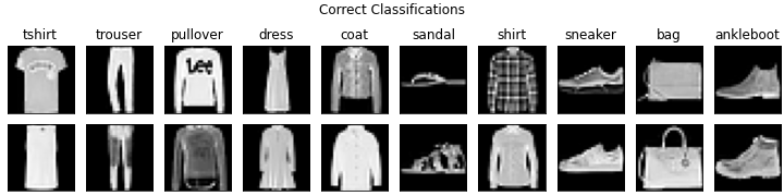
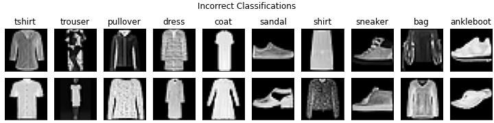
To futher visualize per-class performance, I found two images for each class that the network classifies correctly and two images that it classifies incorrectly. Most of the misclassified pictures are fairly reasonable mistakes; for example, some model/mannequin wears the second "trouser", which is a different perspective than the other images. The picture of the second "ankleboot" is taken at an angle rather than head-on. The first "shirt" looks like an amorphous blob to me. However, there are still some head scratchers, such as the first "trouser" and the sandals.
Visualizing the Network
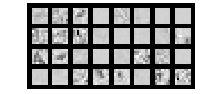
We visualize the first convolutional layer by displaying the 32 filters. Any 7x7 square in the image that roughly matches the shade gets strongly activated, which gives a general idea of what the filter is looking for. With that being said, it is almost impossible to decipher this pixelated mess, which is a theme shared across neural networks in general.
Part 2: Semantic Segmentation
Objective
In this part, we apply convolutional neural nets in the task of semantic segmentation. Rather than assigning a class to an image, we are now to analyze an image of a building and identify its parts (e.g. windows, balconies). We are given a mini facade dataset of 906 training images and 114 test images.
| Class | Color |
|---|---|
| Facade | blue |
| Pillar | green |
| Window | orange |
| Balcony | red |
| Other | black |
Network Layout
For this task, I chained six convolution layers together. I decided against adding affine layers at the end of the network, reasoning that semantic segmentation is more location-dependent than classification. I used ReLU nonlinearities and maxpool layers in the network, and had to upsample to match dimensions with the input image. I used a square filter of size 7 again, simply to keep things constant. Note that the last convolution layer has 5 output channels to match the 5 target classes.
[conv(32) - relu - maxpool(2)] x 2 - conv(64) - relu - maxpool(2) - [conv(64) - relu] x 2 - upsample(8) - conv(5) Training Procedure
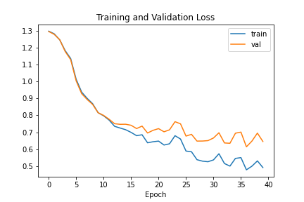
I took the first 795 of the training images as my training set and left the remainder as the validation set. I used a batch size of 15 and an Adam optimizer with learning rate of 1e-3 for the training. I used the standard cross-entropy loss, and ran the training for 40 epochs, which seemed to be where the validation loss starts tapering off.
Evaluating Performance
I use the Average Precision (AP) metric to evaluate the model performance. This metric leverages precision (true positive / true + false positives) with recall (true positive / true positive + false negative). When running over the test, my network's average AP score is 0.583 across all the classes.
When analyzing per-class performance, the wide range of precisions strikes out. In the previous section, the worst performing class ("shirt") was an accuracy of around 13% lower than the next lowest. However, "pillar" is a full 40% lower than the next one. One possible explanation could be that the training images did not have many examples of pillars; after all, it is a decorative element that is not always built in modern architecture. Another explanation could be that pillars could take a wide variety of shapes and sizes, and that the classifier would err on the side of caution and mislabel it as "other".
| Class | Color |
|---|---|
| Facade | 0.744 |
| Pillar | 0.181 |
| Window | 0.748 |
| Balcony | 0.584 |
| Other | 0.657 |
Applying the Network
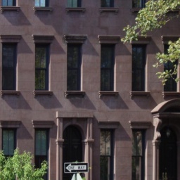
I found a couple images with appropriate building features in my photo collection. After cropping them to the same size as the dataset images and running them through the network, I get the following results.

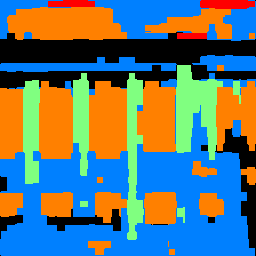
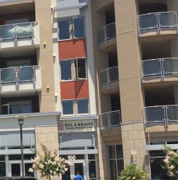
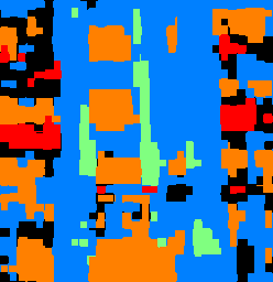
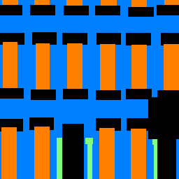
The first set of images is our very own Doe Library. The CNN evaluates the lower and middle horizontal splices fairly well. The windows and exterior facade is labeled correctly. The classifier even got the pillars correct despite its overall 18% average precision. However, the upper splice is misclassifed severely. The roof and sky, normally in the "other" category" has been interpreted as windows and balconies. The network was probably confused by the shadows on the roof, and the sunroof of Doe Library does look a little like a balcony floor. The second image (of a high-end apartment complex) sheds some more light on the network performance. While the windows are generally labeled correctly, the network confused the white paint on the walls as pillars. These false negatives are a reason why the pillar average precision score is so low. The network also missed a column of balconies in the middle, but aside from that and its general messiness, this is a fairly reasonable correspondence result.
Part 3: Conclusion
Overall, this assignment gave me a lot of experience with PyTorch, Colab, and neural nets. Despite currently taking CS182 and having taken CS189 already, this assignment is the first time I had to create a full neural net workflow from scratch. I got to appreciate how time-consuming the training process is (thank goodness for the GPU acceleration) and I barely scratched the surface of optimizing hyperparameters.
With that, there are a couple concepts that I learned from previous classes that I wish I had the time and energy to implement here. One example is cross-validation. We divide the training dataset into many parts and run multiple trials keeping hyperparameters constant with a different section as the validation set. This method reduces codependence across the training set and allows us to use the entirety of the dataset, rather than setting aside 10-15% completely for validation.
The other feature I would've loved to implement is specific to the second part of the assignment. There are other loss functions better suited for semantic segmentation than cross-entropy loss. One such function is intersection-over-union (IOU), which is calculated by dividing the size of the overlapping region by the size of the union of the predicted and ground-truth regions. The reasoning is that the optimizer should worry less about individual pixels (especially on feature borders) and more about holistic overviews. Additionally, taking the average IOU forces the network to treat each class equally, even if one class is underrepresented in the training set. This metric is more closely related to the average precision performance evaluator that we eventually used, and should raise the abysmal "pillar" performance by a reasonable margin. Lastly, it would probably make for cleaner labeling as well.