By Alex Kassil (cs194-26-aca)
Credits to this tutorial for most of part 1.
Here is the code for my dataloader
	transform = transforms.Compose([transforms.ToTensor(), transforms.Normalize((0.5,), (0.5,))])

	trainvalset = torchvision.datasets.FashionMNIST(data_folder, train=True, download=True, transform=transform)
	trainset, valset = torch.utils.data.random_split(trainvalset, [54_000, 6_000])
	testset = torchvision.datasets.FashionMNIST(data_folder, train=False, download=True, transform=transform)

	trainloader = torch.utils.data.DataLoader(trainset, batch_size=4, shuffle=True, num_workers=2)
	valloader = torch.utils.data.DataLoader(valset, batch_size=4, shuffle=True, num_workers=2)
	testloader = torch.utils.data.DataLoader(testset, batch_size=4, shuffle=False, num_workers=2)
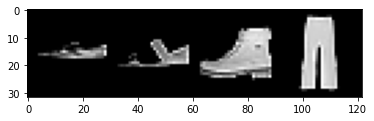
I decided on a 90% 10% train/validation split, as well as normalized the data. I also grouped the pictures together with a batch size of 4 and shuffled the train/validation data. From here we can visualize 4 images, sneaker, sandal, ankle boot, and trouser.
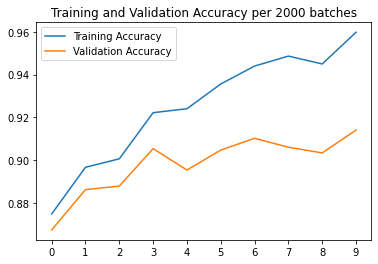
Next was constructing a neural network to train on the train dataset, validate on the validation dataset, and compute a final score on the test dataset. The model takes in 4 1x28x28 images as input, then computes a 5x5 convolution to get to 32 channels, then a relu then a 2x2 maxpool, then another 5x5 convolution to get to 64 channels, then another relu and maxpool, then fully connected layer from a 1024 dimensional vector to 256, relu, 256 to 64, relu, 64 to 10 classes.
----------------------------------------------------------------
        Layer (type)               Output Shape         Param #
================================================================
            Conv2d-1           [-1, 32, 24, 24]             832
         MaxPool2d-2           [-1, 32, 12, 12]               0
            Conv2d-3             [-1, 64, 8, 8]          51,264
         MaxPool2d-4             [-1, 64, 4, 4]               0
            Linear-5                  [-1, 256]         262,400
            Linear-6                   [-1, 64]          16,448
            Linear-7                   [-1, 10]             650
================================================================
Total params: 331,594
Trainable params: 331,594
Non-trainable params: 0
----------------------------------------------------------------
Input size (MB): 0.00
Forward/backward pass size (MB): 0.22
Params size (MB): 1.26
Estimated Total Size (MB): 1.49
----------------------------------------------------------------
From my loss function I used cross entropy loss and for my optimizer I used Stochastic Gradient Descent with a learning rate of 0.001 and momentum of 0.9.
criterion = nn.CrossEntropyLoss()
optimizer = optim.SGD(net.parameters(), lr=0.001, momentum=0.9)
The Final Accuracy achieved on the test set was 90.7% accuracy. Below is the per class breakdown
Accuracy of    T-shirt : 90.30 %
Accuracy of    Trouser : 98.10 %
Accuracy of   Pullover : 88.80 %
Accuracy of      Dress : 92.90 %
Accuracy of       Coat : 83.80 %
Accuracy of     Sandal : 97.30 %
Accuracy of      Shirt : 65.40 %
Accuracy of    Sneaker : 95.10 %
Accuracy of        Bag : 98.20 %
Accuracy of Ankle boot : 97.40 %
Accuracy of Everything : 90.73 %
The shirt class did the worse, but that was because there were a lot of other classes that seemed like shirts, like the pullover, T-shirt, and coat, so these classes had the lowest accuracies.
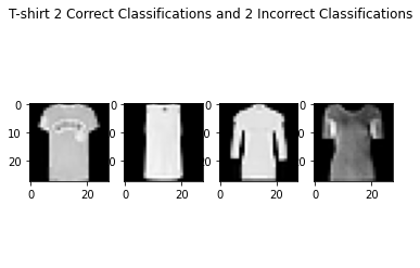
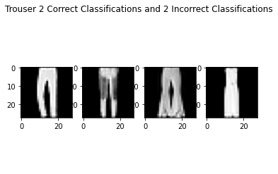
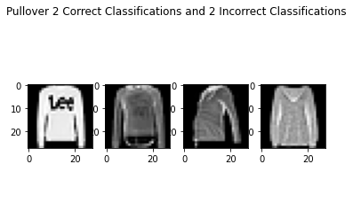
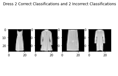
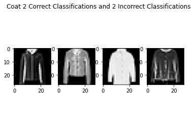
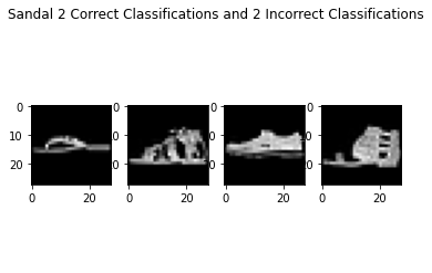
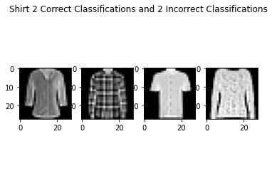
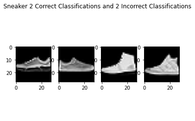
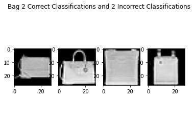
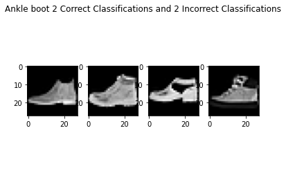
As seen above, the failure cases are quite tough and look similar to the success cases. I imagine even humans would have trouble classifying these from just the pictures alone.
Finally below are the learned filters in the convolutional neural network.
Layer 1


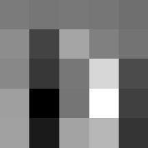


The surprising things from these visualized filters is none of them look symmetrical/like the filters we saw in class, and they all seem unique. There do seem to be some straight black lines which indicate some sort of oriented edge detection.
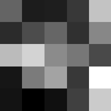
Layer 2


These look pretty similar to the previous filters, but they seem to contain more black
Here is the code for my dataloader
train_data = FacadeDataset(flag='train', data_range=(0,800), onehot=False)
val_data = FacadeDataset(flag='train', data_range=(800,905), onehot=False)
train_ap_data = FacadeDataset(flag='train', data_range=(0,100), onehot=True)
val_ap_data = FacadeDataset(flag='train', data_range=(800,905), onehot=True)

test_data = FacadeDataset(flag='test_dev', data_range=(0,113), onehot=False)
ap_data = FacadeDataset(flag='test_dev', data_range=(0,113), onehot=True)

batch_size = 8
train_loader = DataLoader(train_data, batch_size=batch_size)
val_loader = DataLoader(val_data, batch_size=1)
train_ap_loader = DataLoader(train_ap_data, batch_size=batch_size)
val_ap_loader = DataLoader(val_ap_data, batch_size=1)
test_loader = DataLoader(test_data, batch_size=1)
ap_loader = DataLoader(ap_data, batch_size=1)
I saved 105 images for the validation set, and I also created a one hot encoded set from 100 training samples to quickly compute average AP in addition to loss while training.
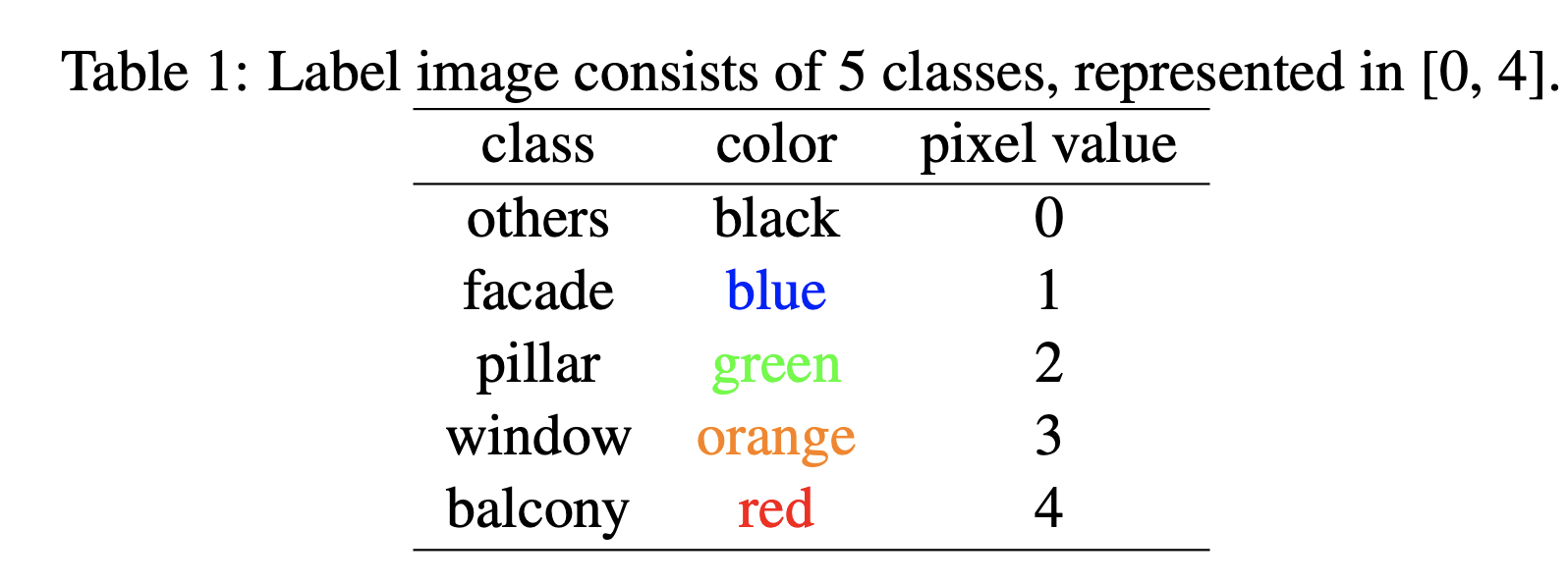

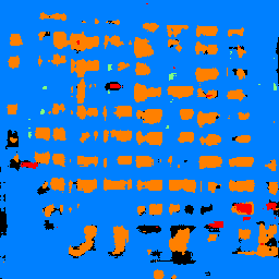
The task for part 2 was to take an image and semantically segment windows, pillars, facades, balconies, from everything else
The neural network for this part was much beefier than the last one and required some extra tricks to get it to achieve a high Average AP score. Main differenes are using batchnormalization and ConvTranspose2d's to undo the MaxPool2d's, since now we didn't want to end up with a 10 dimensional vector but 5 seperate sets of probabilities of class per pixel to then combine into the final segmentation.
----------------------------------------------------------------
        Layer (type)               Output Shape         Param #
================================================================
            Conv2d-1         [-1, 64, 256, 256]           1,792
       BatchNorm2d-2         [-1, 64, 256, 256]             128
              ReLU-3         [-1, 64, 256, 256]               0
         MaxPool2d-4         [-1, 64, 128, 128]               0
            Conv2d-5        [-1, 128, 128, 128]          73,856
       BatchNorm2d-6        [-1, 128, 128, 128]             256
              ReLU-7        [-1, 128, 128, 128]               0
         MaxPool2d-8          [-1, 128, 64, 64]               0
            Conv2d-9          [-1, 256, 64, 64]         295,168
      BatchNorm2d-10          [-1, 256, 64, 64]             512
             ReLU-11          [-1, 256, 64, 64]               0
        MaxPool2d-12          [-1, 256, 32, 32]               0
  ConvTranspose2d-13          [-1, 256, 64, 64]         262,400
           Conv2d-14          [-1, 128, 64, 64]         295,040
             ReLU-15          [-1, 128, 64, 64]               0
  ConvTranspose2d-16        [-1, 128, 128, 128]          65,664
           Conv2d-17         [-1, 64, 128, 128]          73,792
             ReLU-18         [-1, 64, 128, 128]               0
  ConvTranspose2d-19         [-1, 64, 256, 256]          16,448
           Conv2d-20          [-1, 5, 256, 256]           2,885
================================================================
Total params: 1,087,941
Trainable params: 1,087,941
Non-trainable params: 0
----------------------------------------------------------------
Input size (MB): 0.75
Forward/backward pass size (MB): 264.50
Params size (MB): 4.15
Estimated Total Size (MB): 269.40
----------------------------------------------------------------
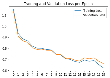
From my loss function I used cross entropy loss again and for my optimizer I used Adam with learning rate of .001 and weight decay of .00001. I stuck with the defaults cause they worked well, even after trying other values and testing on my validation set.
criterion = nn.CrossEntropyLoss()
optimizer = torch.optim.Adam(net.parameters(), 1e-3, weight_decay=1e-5)
AP         = 0.691125830682652
AP         = 0.782778423649354
AP         = 0.207466422931117
AP         = 0.858908038186075
AP         = 0.607026512603763
Average AP = 0.629461045610592
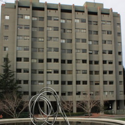
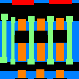
Here is how the network performed on one of the test images
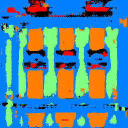
Here it is performing on Evans Hall!