
In this part of the project we are creating a classifier based on Convolutional Neural Networks to classify grayscale fasion images. The neural network takes the image as an input and outputs a vector containing per-class probability. We take the highest probability class as the output from the classifer.
The network for this task is very simple. It contains two convolutional blocks and two fully connected layer at the end.
For each convolutional block, it is consisted by sequential layers of convolution, non-linearity, and a pooling layer to reduce the dimensions.
The structure of the whole network at the end looks like this:
   (1,  32, 32) -> Convolution (5x5, 32 filters)
-> (32, 32, 32) -> ReLU
-> (32, 32, 32) -> MaxPool (2x2)
-> (32, 16, 16) -> Convolution (5x5, 32 filters)
-> (32, 16, 16) -> ReLU
-> (32,  8,  8) -> MaxPool (2x2)
-> (32,  4,  4) -> Fully-connected layer
-> (256)        -> Fully-connected layer
-> (10)            Per-class probability
Training a neural network is basically fitting a very high order function using a lot of data points. The dataset for this task contains 60000 training images and 10000 test images. The training set is split to a group of training data with size 50000 and another group of validation data with size 10000 so that we can monitor the network during training.
The loss function that is being optmized is cross entropy loss and the optimizer used is Adam, with learning rate set to 0.01 and all other parameters to default.
Here's a diagram of training / validation loss against epoch. The blue line is training loss and the orange line is validation loss. The horizontal axis is the number of epochs and the verticle axis is the loss. We trained the network for 20 epochs (20 passes on the full training set), and we see the network converges at about the same time.
| Class | T-shirt/top | Trouser | Pullover | Dress | Coat | Sandel | Shirt | Sneaker | Bag | Ankle boot |
|---|---|---|---|---|---|---|---|---|---|---|
| Accuracy on Test Set | 80 % | 96 % | 74 % | 89 % | 79 % | 98 % | 72 % | 97 % | 97 % | 94 % |
| Accuracy on Validation Set | 88 % | 99 % | 80 % | 96 % | 87 % | 99 % | 87 % | 98 % | 99 % | 96 % |
This is the image of learned network filters on the first layer.
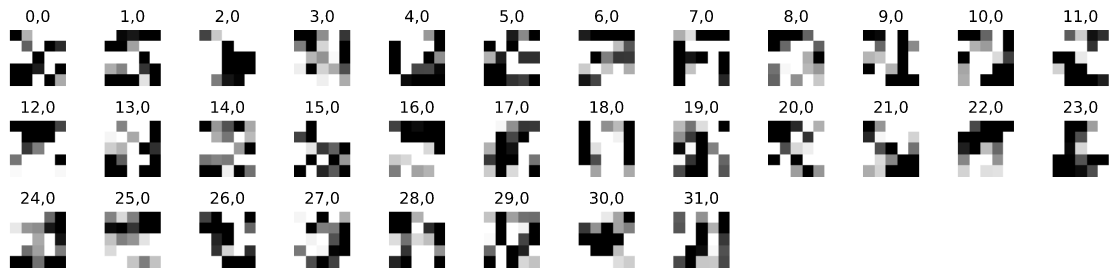
Unlike weights from typical deeper network, the weights from this network seems strange and have very strange patterns. This may be that the layer depth is too low and the image is too low-res that the network learned more higher order features / shapes from the original image.
This part of the project is to build a segmentation network that labels images of building facades with different surfaces (windows, pillars, etc.). It takes a color image as an input, and outputs a segmentation image. This can be understood as a image transformation / generation model where an real image of facade is turn into abstract image os blobs. However it is more so usually understood as a classification problem, just this time the classfier outputs the class on a per pixel basis.
Upon some research, there are two architecture that is said to be very good at image segmentation. The first one is Unet (O Ronneberger, 2015), which is originally used for segmenting medical images with a binary class output. The second one is SegNet (V Badrinarayanan, 2015), which is a segmentation network that is a multi-class segmentation network that operates on natural images.
Both of these networks are encoder-decoder networks, which basically consists of two parts. The first part is an encoder, whose job is to "encode" a image into a vector or set of features. The encoded features than is fed into the "decoder" to turn the features into a final image. The features are usually "bottlenecks" of the network, so that the network can be trained to represent the images with a "latent space information" that is usually much smaller than the original image, somewhat like a image compression / restoration process.
Both Unet and SegNet has residual path where the encoder passes some of the information other than the latent space vector to the decoder for higher resolution output / more precise or local data. The difference between these networks is Unet passes the higher resolution features to the decoder and concat them with the decoded features, like most residual network do. SegNet on the other hand passes the max-pooling indices to the decoder to restore higher resolution information.
I tried both networks on this task, however none of them worked well. Both of them can't converge onto a lower loss (they all converged at about mAP=0.3). No matter how many epochs are fed into the network, it just doesn't seem to converge. Initially I think the problem could be the dataset is not large enough to train a encoder-decoder network, so I performed data augmentation (the dataset are flipped horizontally). This does not yield a visible improvement. The second possible problem is that our loss function are not suitable for this task. The cross-entropy loss used in this task assumes that the class are balanced so that the probabililities for each class is similar. However for image segmentation tasks it's natural that the labels are not balanced at all. I tried to use inverse frequency weighting, where the per-class frequency is computed on the training set, and it reveals huge inbalance in the dataset. However, using this weighting does not bring a huge improvement to the result.
All previous attempts scrapped, and it's time for new thoughts.
As I introduced in the overview part, this task can also be understood as a classification problem, instead of a image generation problem. If we can run a classifier on small windows of the network and produces a per-pixel class result, we can solve this task. We know how to build such a detector: we can simply strip away the fully-connected layers of a detetion network, and put convolutional layers at the end to produce a per-pixel probability.
The network I chose is ResNet, for its simplicity in design and relatively low amount of weights due to the use of small filters. Also ResNet is known to be very easy to train because of its residual connections serves as a "high-way" for gradients.
A typical ResNet looks like this:
   input
-> Conv2d
-> ResNet block
-> ResNet block
-> ResNet block
...
-> ResNet block
-> ResNet block
-> ResNet block
-> Fully-connected layer
-> Fully-connected layer
-> output
where each block looks like this:
-> Conv2d
-> Batch Normalization
-> ReLu
-> Conv2d
-> Batch Normalization
-> ReLu
...
-> Batch Normalization
-> Residual Connection
-> ReLu
For this task, I removed the fully connected layer, and used 4 layers of convolution per block. Each layer has a 3x3 filter, and the feature depth grows per two blocks:
   (3,  256, 256) input
-> (3,  256, 256) Conv2d (7x7)
-> (16, 256, 256) ResNet block (3x3, 4 convolutions)
-> (16, 256, 256) ResNet block (3x3, 4 convolutions)
-> (32, 256, 256) ResNet block (3x3, 4 convolutions)
-> (32, 256, 256) ResNet block (3x3, 4 convolutions)
-> (64, 256, 256) ResNet block (3x3, 4 convolutions)
-> (64, 256, 256) ResNet block (3x3, 4 convolutions)
-> (64, 256, 256) Conv2d (1x1) (Baiscally a fully-connected layer that operates on per-pixel)
-> (5,  256, 256) output
Also because the imbalanced dataset, the loss function is changed to "dice loss", which measures the distance between images directly instead of calculating the softmax.
This architecture turns out to be super succesful on this task. Only after a single epoch (without dropout and data-augmentation), the network already performed better than the best result previously obtained with encoder-decoder networks.
After some careful observations, I find that the dataset's segments are all rectangles. If we think about the process of a convolutional network as applying filters onto images and higher dimension images of features, in theory we can get away with two low rank kernels instead of a huge square kernel. In ResNet's design, the very deep network with 3x3 filters is to use as few parameters possible while still be able to deal with large scale features. I replaced the convolutional layer in each ResNet block with two convolutions, one verticle and one horizontal:
-> Conv2d (1x7)
-> Conv2d (7x1)
-> BN
-> ReLU
...
Because we can use much wider kernels, I reduced the convolutional layers per ResNet block to 2, and in theory we are covering a even larger area so larger features can be considered. We also decreased the parameters by about a third ( vs ). The new design achieved similar results with lowered amount of parameters. The final architecture looks like this:
   (3,  256, 256) input
-> (3,  256, 256) Conv2d (7x7)
-> (16, 256, 256) SegResNet block (7x1 & 1x7, 2 convolutions)
-> (16, 256, 256) SegResNet block (7x1 & 1x7, 2 convolutions)
-> (32, 256, 256) SegResNet block (7x1 & 1x7, 2 convolutions)
-> (32, 256, 256) SegResNet block (7x1 & 1x7, 2 convolutions)
-> (64, 256, 256) SegResNet block (7x1 & 1x7, 2 convolutions)
-> (64, 256, 256) SegResNet block (7x1 & 1x7, 2 convolutions)
-> (64, 256, 256) Conv2d (1x1) (Baiscally a fully-connected layer that operates on per-pixel)
-> (5,  256, 256) output
We used Adam optimizer with learning rate of , with a batch size of (a limitaion on the GPU memory). As this network utilizes residual learning, the network trains very fast. Data augmentation is used on the training set (images and labels are fliped horizontally).
The blue line here is the vanilla ResNet, the green one is the modified ResNet. Due to data augmentation, we can see that the validation loss is considerablly lowered, while the loss on the training set suggests that the modifications to the network does not degrade the performance.

We can see that at the end of training out network is starting to over-fit, but we can probabily still improve our performance a bit by training for more epochs. We can probably get another uplift in performance if dropout is used.
At the 20-th epoch, the network is able to achieve a validation loss of 0.21, and the AP on the test set is:
AP = 0.7630981507127597
AP = 0.8330740872849791
AP = 0.1761574408426417
AP = 0.879061284348575
AP = 0.6691120915461404
At the end of training (epoch=140), it reached a validation loss of 0.13, and the AP on the test set is:
AP = 0.7277495011360715
AP = 0.8114285717300367
AP = 0.23289149428261735
AP = 0.8736086904440306
AP = 0.644270659953635
The mean-AP on training set is . The precision on pillars and balconies are very high compared to a simple CNN or a encoder-decoder network where we are seeing a precision smaller than . Considering the dataset only contains very small amount of examples of these two classes, this is very amazing result.
Here is a image found online:

And here's the output result:
We can see that the network is able to capture the approximate locations of the segment. However the background facades are not very clean, likely due to the scale of the image being too large compared to the training data the network has seen.
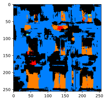
Here's a more challanging facade, the MIT's CS building:
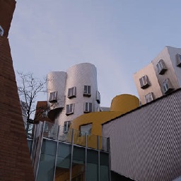
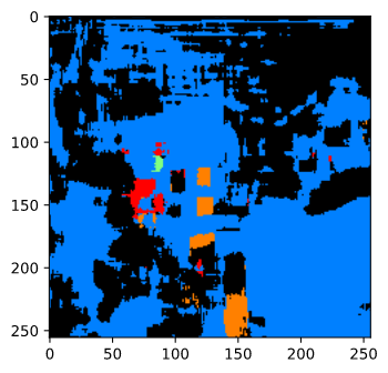
We can see that it managed to find several small windows in the center row, but the curved facade and exotic shapes confused the network a lot.