HW 4: Neural Networks

Part 1: Image Classification

We attempt to train a Convolutional Neural Network (CNN) on the FashionMNIST dataset to classify items of clothing.

Below are examples from the dataset, taken from the FashionMNIST website.

There are 10 classes: T-shirt, Trouser, Pullover, Dress, Coat, Sandal, Shirt, Snaker, Bag, and Ankle Boot. Each image is grayscale, and \(28 \times 28\) pixels in size.

Network Architecture

Our network architecture is as follows:

Training & Hyperparameters

We split the train set of FashionMNIST into a 50000 image train set and a 10000 image validation set.

We use the following hyperparameters:

• Optimizer: Adam
• Learning rate = \(5 \times 10^{-4}\)
• Weight decay = \(10^{-3}\)
• Epochs = \(8\)

Results

We report a validation accuracy of \(90.03 \%\), after tuning the network architecture and hyperparameters.

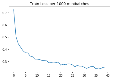
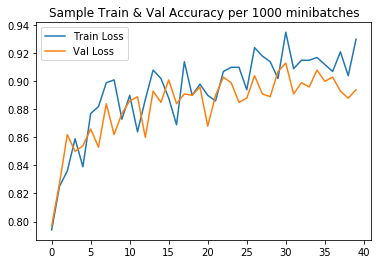
We display training loss and sample train and validation accuracy every 1000 minibatches. The accuracy is computed over randomly drawn samples of size 1000 from the training and validation sets.

We report per-class accuracy statistics:

Accuracy of T-shirt : 84 %
Accuracy of Trouser : 97 %
Accuracy of Pullover : 89 %
Accuracy of Dress : 93 %
Accuracy of  Coat : 85 %
Accuracy of Sandal : 95 %
Accuracy of Shirt : 61 %
Accuracy of Sneaker : 98 %
Accuracy of   Bag : 97 %
Accuracy of Ankle Boot : 92 %

We also include a confusion matrix to visualize misclassifications. The index corresponds to the position of the class in the list above.

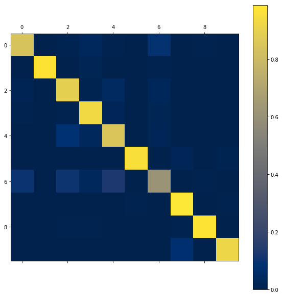
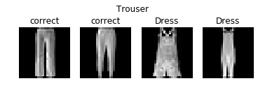
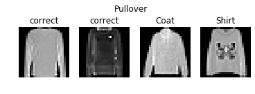
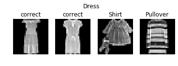
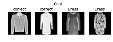
Element \(C_{ij}\) of the matrix corresponds to examples that are in class \(i\) but are misclassified into class \(j\). As we can see here, the poorest performers, T-shirt, Coat, and Shirt all are frequently misclassified to visually similar classes: T-shirt and Shirt are frequently mixed, and Shirt images are mistaken as Coat, Pullover, and T-shirt.

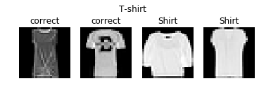
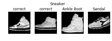
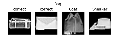
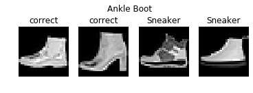
We also display correctly- and incorrectly-classified examples for each class. This further shows some of the visual ambiguity of the classes discussed above.

We also display the first convolutional layer's filters.

We observe several filters that look like Derivative of Gaussian filters, with dark regions on one half of the image and lighter features on the other half, such as the 1st image in the 4th row, or the 4th image in the 2nd row.

Lastly, we report a test set accuracy of \(89.57\%\).

Part 2: Semantic Segmentation

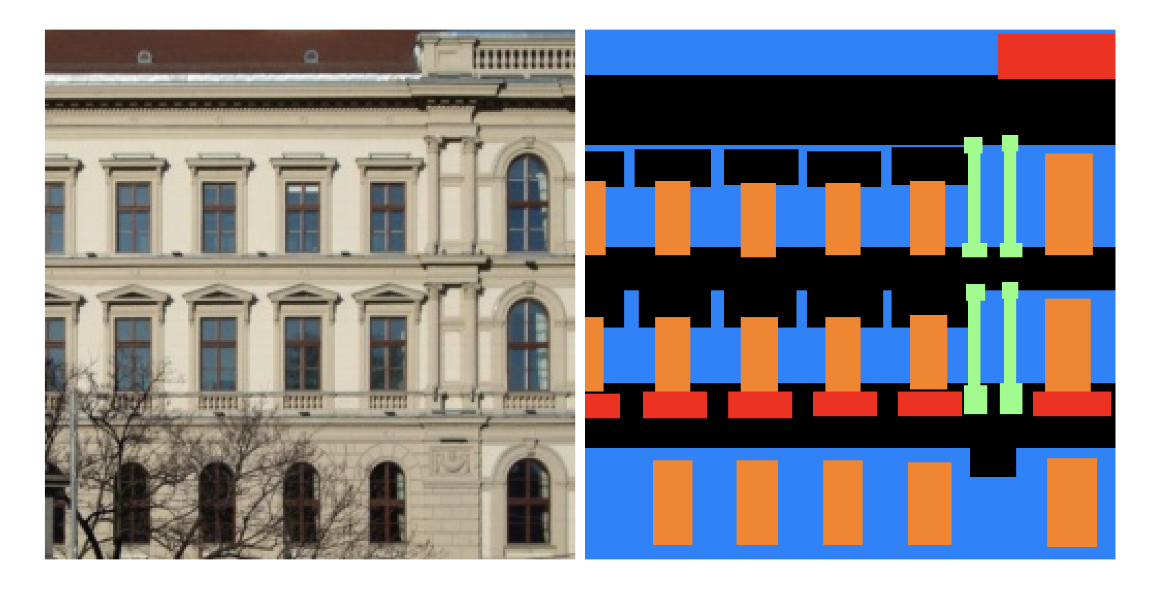
We attempt to train another network to perform semantic segmentation on a provided dataset of building facades. The dataset images and labels look like the following image, taken from the spec:

We seek to classify each pixel in a \(256 \times 256\) pixel RGB image into one of 5 possible classes, shown below in a table taken from the spec:

Network Architecture

Our network architecture is as follows:

We take inspiration from the 2015 paper U-Net: Convolutional Networks for Biomedical Image Segmentation which also performs semantic segmentation. It also repeatedly doubles the input volume channel count while halving its spatial dimensions using successive \(3\times3\) convolutional layers and max pooling layers, and then upscales it in a similar fashion using learned transpose convolution layers and traditional convolutional layers. We do not implement the multi-level feature copying approach, although it is possible that it could improve results further.

Training & Hyperparameters

We split the 905 training images into a 805 image train set and 100 image validation set.

We use the following hyperparameters:

• Optimizer: Adam
• Learning rate = \(2 \times 10^{-4}\)
• Weight decay = \(5^{-5}\)
• Epochs = \(30\)

Results

We report an average validation mean average precision of \(0.5965\), after tuning the network architecture and hyperparameters. The breakdown of the average precisions over the 5 classes (others, facade, pillar, window, balcony) is as follows:

AP = 0.6985607901119048
AP = 0.786236119580659
AP = 0.19339308281423281
AP = 0.8330665282198559
AP = 0.4711577114896065

While this exceeded the 5-6 conv layer recommendation, I was able to achieve a validation mean average precision of as high as 0.65 by inserting an additional \(3\times 3\) convolutional layer with the same channel count immediately before each max pooling or transpose convolutional layer. This was done in the U-Net paper linked above.

We immediately notice a trend of the network struggling to identify pillars and balconies, which are smaller, less common features.

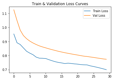
We show train and validation loss curves per epoch:

We display some examples from the validation set:

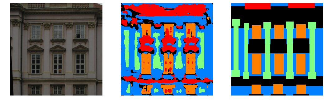
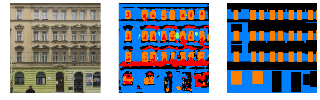
Some interesting observations:

• The other class is often labelled inconsistently, sometimes being applied to image artifacts (regions of black), and sometimes to buildings that aren't the primary one, and sometimes parts of the primary building itself. However, it does not often fully cover everything, which confuses the network.
• The network often predicts regions as pillars that look visually similar to labelled pillars, even if they are labelled as facades. It appears sensitive to narrow flat surfaces in between windows that have a defined edge.
• The network frequently overpredicts areas below windows as balconies and appears to use shadows as a strong marker for balconies.

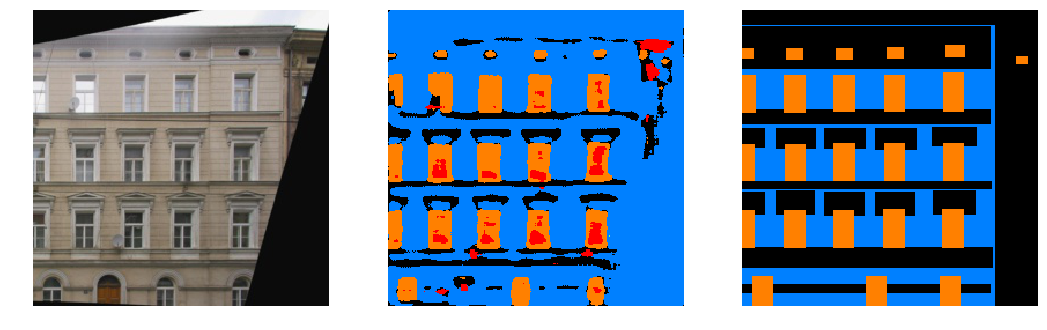
We also display the network predictions on an image from outside the dataset:

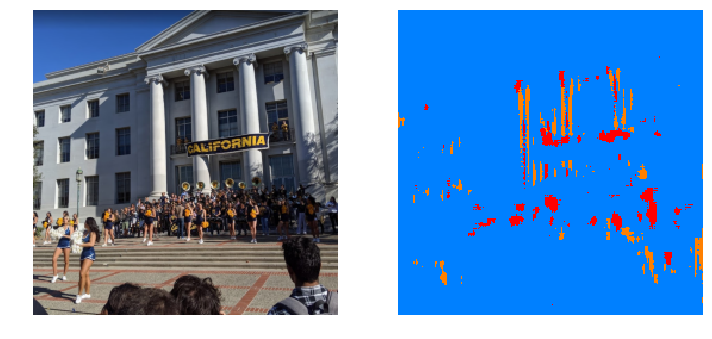
The network completely fails to classify this image. There are several aspects of it that make it difficult to classify, including:

• Geometry that is not aligned. All training images have had an affine warp applied to them to straighten out the windows, columns, etc.
• People. The network preducts those as balconies or windows.
• Prominent lighting differences.

This suggests that the network may have overfit more broadly to some dataset characteristics including alignment and the general image cleanliness.

Finally, we report a test set mAP of \(0.5794\).