Part 1: Image Classification
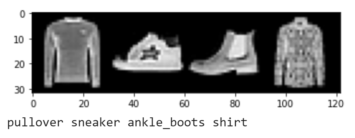
Before we trained our network, we used a data loader to retrieve the input data. Above is a peek into what each testing batch looks like. We decided to test in groups of four.

We decided to train our network over 15 epochs with a learning rate of 0.001
and using a batch size of 128 (train and validation). The architecture of the
network involves 2 convolutions with channels 32 (kernel = 5) and 64 (kernel = 5), both followed by
ReLU and max pooling. Then, in the fully connected layers, we used 1024,
120, and 84. The class and overall accuracies are shown in the table below.
From the graphs above, we see that as the epochs increased, training accuracy and loss
were better than that of the validation. This suggests that our network is overfitting.
Two correct examples are shown to the right, and two incorrectly labeled examples
are shown to the left. The class that they belong in is shown by the "Actual" column.
The testing accuracies are shown in the leftmost column.
Here are the validation accuracies:
Overall: 91.044
t_shirt : 87 %
trouser : 97 %
pullover : 90 %
dress : 94 %
coat : 87 %
sandal : 93 %
shirt : 71 %
sneaker : 95 %
bag : 97 %
ankle_boots : 95 %
Though the performance is similar, we see that there's slightly better performance in
classes in validation, though the shirt category continues to suffer. This may be due to the
fact that validation was split via a SubsetRandomSampler, so some trained data may be repeated
in the data for class accuracies.

We see that the network performs the best for Bags and Trousers, both at 97%.
However, it struggles to identify Shirts, only scoring 68%. This may be because the Shirts category is
very broad and may include items of clothing that are similar to other categories. From
the examples, we see that the network tended to mistidentify Shirts as T-Shirts, high-top
Sneakers as ankle boots, and overalls in the Trouser category as dresses.
After looking more closely, I now realize I'm not sure what a T-shirt is anymore. The first
mis-identified Shirt looks like a T-shirt to me and the tank top in the T-shirt category
was something that I thougth would belong in Shirt.
Visualizing the filters
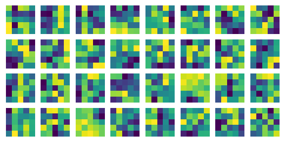
To better understand how the network is learning, we decided to visualize the filters as determined by the weights from the first convolutional layer. Larger values within each filter are shown with brighter values (toward yellow).
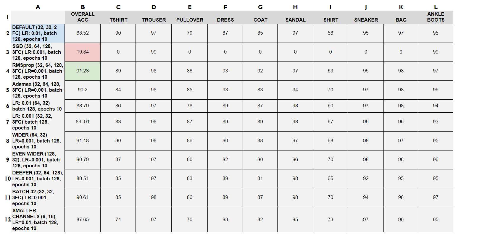
1.1: Experimenting with hyper-parameters
Before we settled on this network, we did perform some experiments with changing the
learning rates, batch sizes, architecture, and optimizers. Here are the class and overall performances
of each.
We see that using RMSprop with a deeper network and smaller learning rate performed the best and that SGD optimization resulted overfitting to the Trousers and Ankle Boots. This may be due to the fact that our batch sizes were really large, causing certain features to be excluded. Generally, larger channel sizes produced better accuracies, though deeper nets resulted in large overfitting.
Part 2: Semantic Segmentation
In this part, we allow the network to make decision on each pixel to display a certain color using the Mini Facade dataset. We designed the network based off of UNET, which was created for biomedical image segmentation, where training sets are limited in size. Since our facade dataset is similarily small, we thought that UNET could be a good place to draw inspiration from.
We chose to make our network have 5 convolution layers and 3 transposed convolution layers. Channels 64 (kernel = 3), 128 (3), 256 (3), 512 (3) were designated for the first four convolution layers, each followed by ReLU and max pooling except for the first layer. 3 transposed convolutions (kernels: 3, 3, 5, output padding 1) followed with 1 more convolution with output 5 (# of classes) and ReLU. Kernel sizes were picked such that the smallest image size would be 30x30.
We chose to use a learning rate of 1e-3, weight decay of 1e-5, batch sizes of 32, and 80 epochs. Similar results were accomplished by using smaller batch sizes (10) and 10-20 epochs.

We see that the validation loss heavily deviates from the training loss as the epochs increased, indicating overfitting. To combat this, we decided to try lower learning rates and smaller batch sizes. The average precision can be seen below.
AP = 0.5144015916006488
AP = 0.6655199157812598
AP = 0.044730906176792685
AP = 0.7499151291135202
AP = 0.40716600573957046
Total: 0.476
2.1: Experimenting with hyper-parameters
We also looked at networks that performed with similar accuracy in less epochs. The testing loss of these networks were also better.
learning rate 0.00088, epochs 10, batch size 10
Calculating Average Precision
AP = 0.5684381492133768
AP = 0.6530035841707463
AP = 0.058622461809989104
AP = 0.7305726765444372
AP = 0.3084583222115016
Total: 0.462

We see significantly less overfitting, though it converges to about the same average precision.
Learning rate: 0.00088, epochs 20, batch size 10
AP = 0.5616283544878281
AP = 0.6323685950180747
AP = 0.06300031998970657
AP = 0.6513815101728105
AP = 0.4635128700430303
Total: 0.473
learning rate: 0.0008, epochs 15, batch size 10
AP = 0.5297797145550298
AP = 0.6617536893884522
AP = 0.05439818835798544
AP = 0.67628196761542
AP = 0.4446927352443966
Total: 0.472
2.2: Looking at the results

After training and testing, here's the fun part. What kinds of cool images does our network produce? Apparently very abstract blobs of orange.
This network does a very good job when it comes to identifying windows, so much to the point that it thinks everything is a window, as you can see in the images above. It also did a fairly decent job of identifying the pillars on the second example even though its overall accuracy for pillars is poor (6%), but there's just a lack of blue, or facade in most of these outputs.
Looking through the outputs I found the image with the Tree obstructing the building to be very interesting. We see a huge blob of red, the outline of which is suspiciously similar to the tree. Though there was no building to be labeled where the tree is from our perspective, the network was able to take neighboring colors (though misidentified) and stick them there.
Overall, the most important thing I learned from this project is that identifying features of objects can often be brought out through different masks. A combination of these "views" can then be generalized to a class.