In this assignment we will be using convolutional neural networks to perform image segmentation and image classification tasks. We will be classifying images from the Fashion-MNIST dataset with a traditional convolutional network and segmenting images from the mini Facade dataset using a fully convolutional or U-Net architecture.

We will be using the Fashion-MNIST dataset for this classification task. In the creation of this network, I tried a few designs but quickly settled on the final design shown below as it achieved greater than 90% accuracy. My other primary design that I had before this was exactly the same, but had one fewer fully connected layer after the convolutional layers. Even this relatively simple network was able to achieve great results!

The only other parameters I touched at all were the parameters for learning rate and weight decay. The default values performed pretty well, but I was able to achieve slightly better accuracy and convergence with the learning rate of 0.0001 (smaller than default) and weight decay of 0.001 (larger than default).

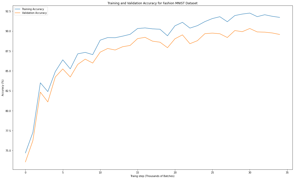
For this net, I trained on 10 epochs and was able to achieve a training accuracy of 92.775% and a test accuracy of 90.63%. The plot below shows the training and validation accuracy across 10 epochs (each step in the plot is 1000 batches).

We can also examine the in class accuracy for each of the 10 classes present. This is within the test set after 10 epochs of training. We can see that by a fairly large margin the hardest class to predict at least for this net is shirts. The next two hardest are T-shirt/tops and Pullovers.

  Accuracy of T-shirt/top: 88%
  Accuracy of Trouser: 97%
  Accuracy of Pullover: 84%
  Accuracy of Dress: 93%
  Accuracy of Coat: 99%
  Accuracy of Sandal: 97%
  Accuracy of Shirt: 66%
  Accuracy of Sneaker: 95%
  Accuracy of Bag: 98%
  Accuracy of Ankle boot: 96%

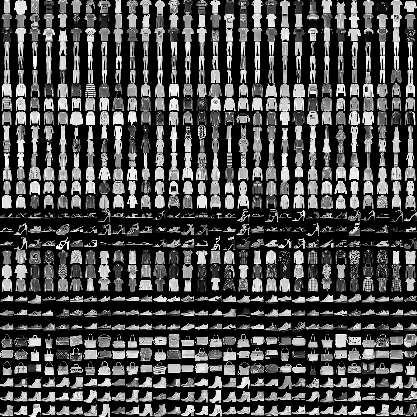
We can try to visualize some of the images that our net predicted correctly and where our net predicted incorrectly. We do this for two images in each of the classes.

Finally we can visualize the learned filters of the convolution. Here we visualize the 64 filters from the first convolution of our final net, shown in no particular order.

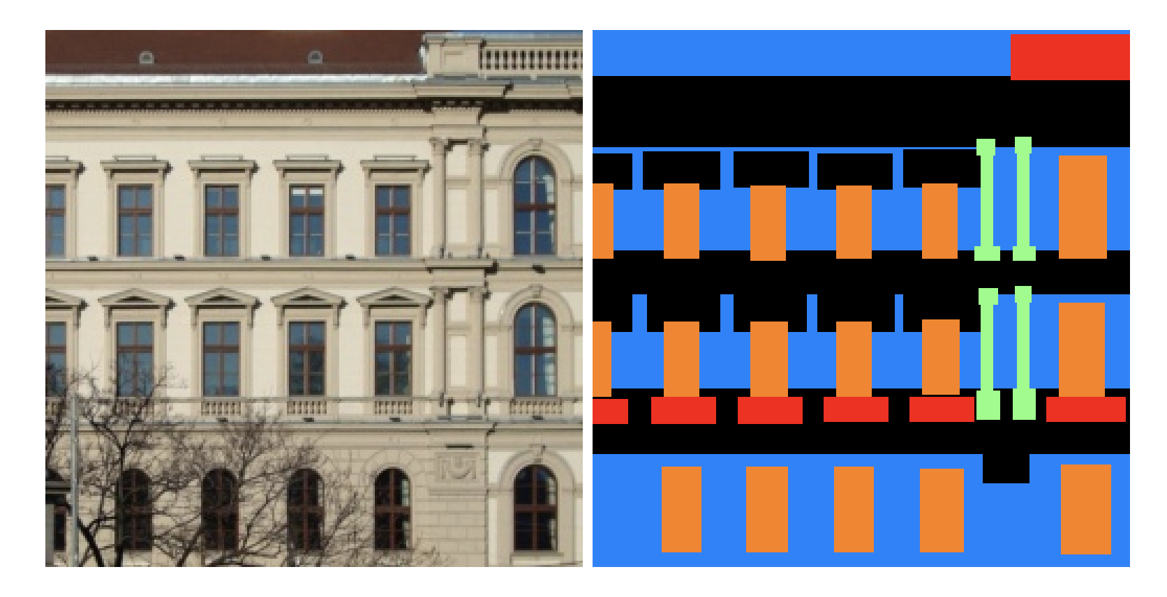
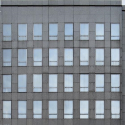
Here we will train a semantic segmentation network. The function of this network will be to input images that are of a specific dataype then segment those images into different classes. For us, we will be taking in images of facades, and we will be segmenting those in the classes of facade, pillar, window, balcony, and others. For this, I followed the U-Net design as can be found in this paper.

Taking this design as a baseline, the main change that I made is I used fewer convolutions at each layer of the U-Net and I also had fewer layers of the U-Net. After implementing this stripped down the design the performance I got was pretty good, thus I did not do any additional hyperparamter tuning. I remained with default values for the optimizer etc. The full network architecture can be visualized in the following diagram.

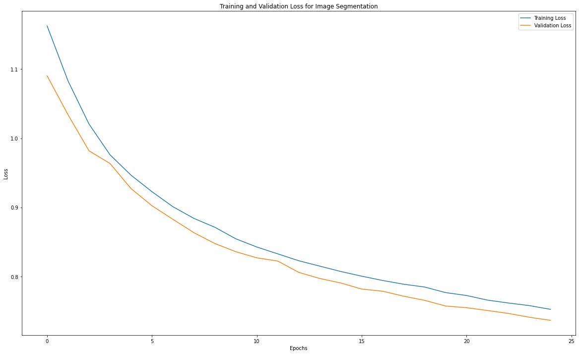
I trained this network for 25 epochs, with a training / validation split of 80% / 20%. The following plot shows the training and validation loss over those 25 epochs. We can see that it appears that the network still has not converged completely, but the results from this net were still sufficiently good, so I opted to not train for a longer time.

After training for 25 epochs the following shows what levels of average precision or AP we were able to achieve for each of the classes, and then in aggregation.

  AP for others: 0.6876688299763116
  AP for facade: 0.7650599058046677
  AP for pillar: 0.12516525322248068
  AP for window: 0.8233394634244902%
  AP for balcony: 0.4205180347113103
  AP for ALL CLASSES: 0.56435029742

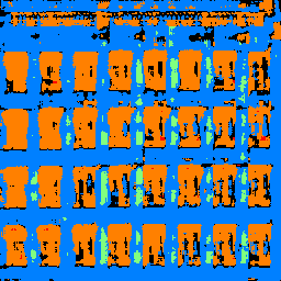
We can try to use the image segmentation network on our own input images to see how it does. Below are the results from an image of my own choosing.