Classification and Segmentation
Steven Cao / cs194-26-adx / Project 4
In this project, we explore the use of Convolutional Neural Networks (CNNs) for image processing. Our tasks will be classification and segmentation. All experiments were run on Google Colab and took about 1 hour each.
Classification
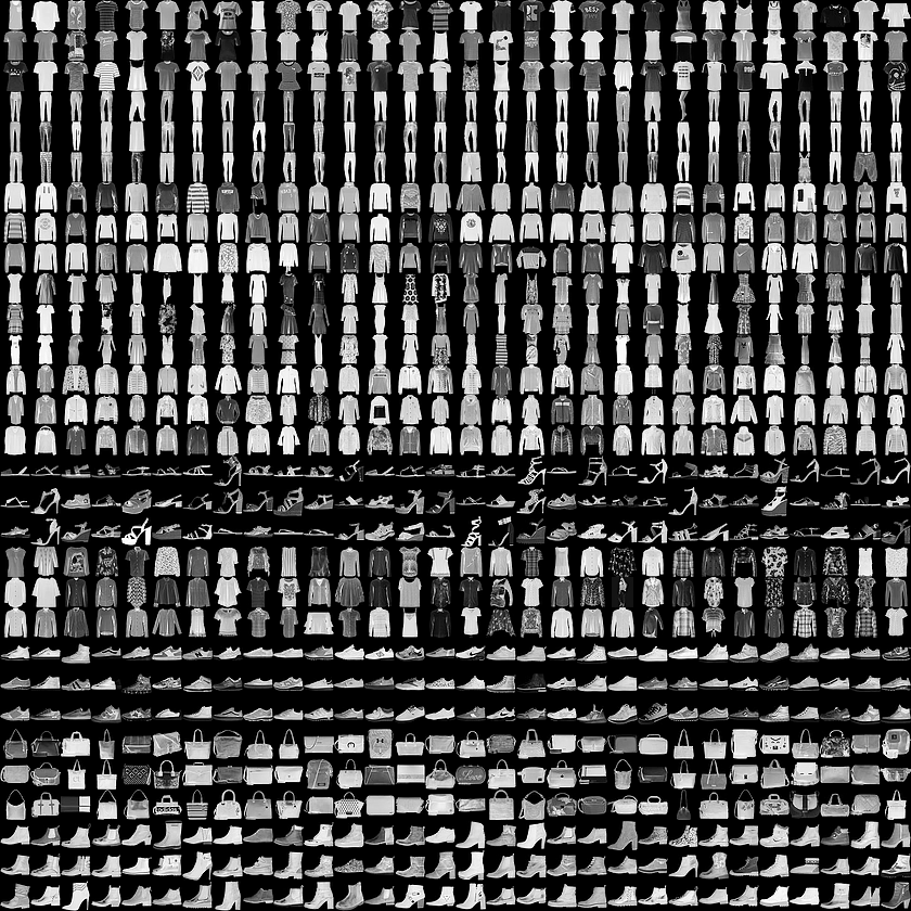
In this section, we will use CNNs to perform classification on the Fashion MNIST dataset, which has 60,000 training examples and 10,000 test examples consisting of 28x28 grayscale images of clothing. The CNN is tasked with determining whether the image is a t-shirt/top, trouser, pullover, dress, coat, sandal, shirt, sneaker, bag, or ankle boot. Below are some example images, taken from the dataset's github page.
As my architecture, I used a simple CNN with four convolutional layers, followed by two fully-connected layers. Each convolutional layer had hidden size 32, filter size 5x5, and padding size 2x2. Each convolutional layer also had a skip connection, followed by a ReLU activation. The second and fourth layers were followed by 2x2 max-pooling. The first fully-connected layer projected down to dimension 128, and the second projected down to 10, the number of classes.
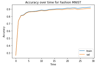
The model was optimized using cross-entropy loss and the Adam optimizer with learning rate 0.001, batch size 1024, and 10 epochs, which took about an hour. The final training and validation accuracies were 0.926 and 0.906, respectively. Below, we show the accuracy curve during training.
Next, we report per-class accuracy on the validation and test set, ordered by accuracy. The four hardest classes are shirt, coat, t-shirt/top, and pullover. One possible explanation is that these classes are easy to confuse with one another.
| Class | Validation Accuracy | Test Accuracy |
|---|---|---|
| Shirt | 0.761 | 0.719 |
| Coat | 0.781 | 0.765 |
| T-shirt/top | 0.809 | 0.812 |
| Pullover | 0.912 | 0.893 |
| Dress | 0.915 | 0.922 |
| Ankle boot | 0.960 | 0.959 |
| Sandal | 0.970 | 0.973 |
| Sneaker | 0.971 | 0.976 |
| Bag | 0.980 | 0.983 |
| Trouser | 0.984 | 0.975 |
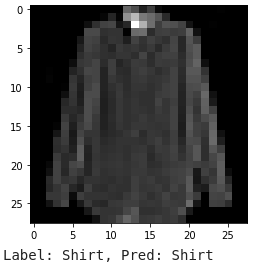
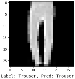
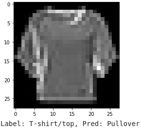
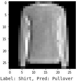
To get a better idea of what our model is doing, we also display some example images that were correctly or incorrectly classified, as shown below. In the two wrong predictions, the model confuses a T-shirt for a pullover, as well as a shirt for a pullover. I can forgive the model because pullovers and shirts look pretty similar.
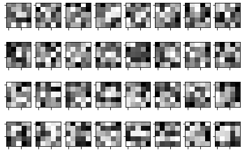
Finally, let's visualize the learned filters to see if anything recognizable emerges. Below, we show the 32 filters for the first convolutional layer. It seems difficult to discern any recognizable structure from them.
Semantic Segmentation
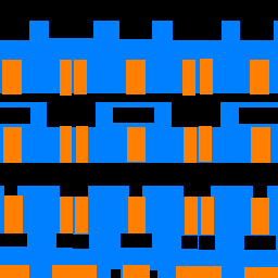
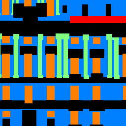
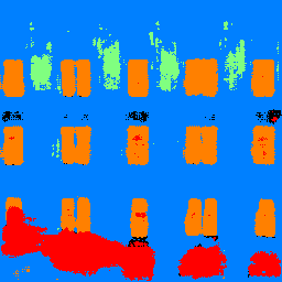
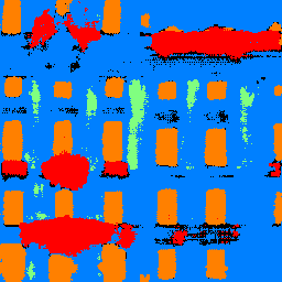
Next, we perform semantic segmentation on the Mini Facade dataset, a dataset with building facades, where each pixel is either a facade (blue), pillar (green), window (orange), balcony (red), or other (black). Below, we show two test examples from the dataset.

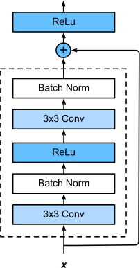
For this task, we use a somewhat more complex architecture. The architecture is inspired by U-Net, a popular architecture for biomedical segmentation, but is a bit simpler. As a basic building block, we will use the residual layer from the famous ResNet, depicted below in a figure from the Dive Into Deep Learning textbook.
At a high level, the model first downsamples the image, then upsamples it. Furthermore, there are connections between the downsampling and upsampling steps. All convolutional layers use padding to keep dimensions the same. Specifically, the architecture is as follows:
- Use a 7x7 convolutional layer to go from 3 to 16 channels.
- First, we will downsample:
- Apply a residual layer with hidden dimension 16. Save the output.
- Apply a 2x2 max-pooling layer, and keep the indices for unpooling later.
- Apply a convolution to go from 16 to 32 channels. Also apply batch norm and a ReLU.
- Repeat step 2, reducing the image size by half again and doubling the hidden dimension again (from 32 to 64).
- Apply a residual layer with hidden dimension 64.
- Now, we will upsample, which applies the downsampling steps in reverse:
- Apply a convolution to go from 64 to 32 channels. Also apply batch norm and a ReLU.
- Apply a 2x2 max-unpooling layer using the indices from the downsampling step.
- First, concatenate the saved output from step 3 to the image (so we now have 64 channels again). Then, apply a residual layer with hidden dimension 32, where the first convolution projects back down to 32 channels.
- Repeat step 5, doubling the image size again and halving the hidden dimension (from 32 to 16).
- Finally, use a 1x1 convolution to go from 16 to 5, the number of classes.
The idea behind the architecture is that by downsampling and then upsampling, the network is forced to compress the input and then decompress. However, one drawback of downsampling is that we lose spatial resolution. Therefore, the connections between the down- and up-sampling steps are meant to preserve fine-grained information.
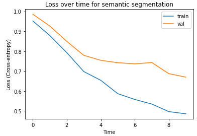
For training, I used the Adam optimizer with with a learning rate of 1e-3 and weight decay 1e-5, and I used cross-entropy loss. The model was trained for 10 epochs with batch size 8, which took about 1 hour, resulting in a final test set average precision of 0.762. Below, we show the training curve. It seems the model has not converged yet, but I stopped at 10 epochs because Google Colab had a time limit. There also seems to be some overfitting, which suggests that perhaps more regularization would helpful.
Below, we report the per-class average precision in ascending order. It seems like the model does reasonably on all classes except pillars.
| Class | Test Set Average Precision |
|---|---|
| Pillar | 0.201 |
| Balcony | 0.631 |
| Other | 0.716 |
| Facade | 0.796 |
| Window | 0.875 |
Below, we show two example outputs. The model seems to be doing the right thing, but the segmentation boundaries are not sharp. It also rarely reports other (black). In the first example, the model confuses shadows with balcony (red). Also, in the second image, the model labels some objects that seem to be balconies (red), but are not labeled as such in the ground truth.
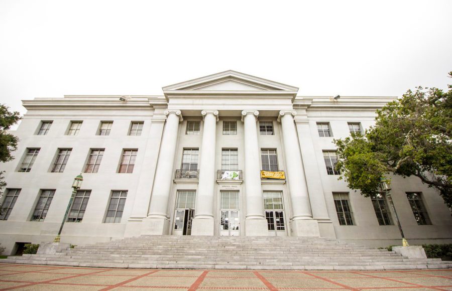
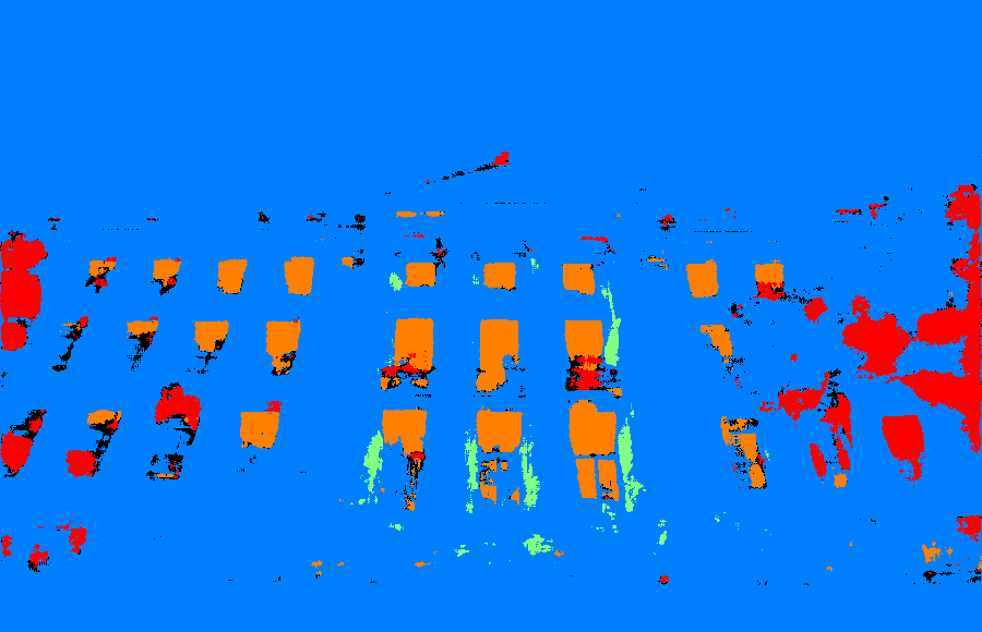
I also tried using the model on a picture of Sproul Hall, as depicted below. The model seems to do quite well, which is promising. It does classify the trees as balconies (red), perhaps because it did not see trees in the training data. The model also continues to label pixels as facade (blue) instead of other (black).
Conclusion
It was cool to see the power of CNNs in action. I am always impressed by how easy it is to train neural nets using Pytorch and how much of the process is implemented and hidden from the programmer (like autodifferentiation, optimization, etc.). It's also nice how we can get reasonable results by using Colab (which is free for anyone to use) with train times under an hour. The ease of use and availability of moderate compute point to how accessible deep learning has become nowadays.