Part 1: Image Classification
Overview
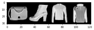
In this section, we use a CNN to classify Fashion MNIST dataset, which has 10 classes with 60000 trainining images and 10000 test images. Below are some images from the dataset:
|
Implementation Details
Overview: The network consists of two convolutional layers, each followed by a ReLU and Max Pool Layer. It is then connected with two FC layers, with the first followed by ReLU. We used cross entropy loss and Adam as the optimizer with learning rate of 1e-3 and a weight decay of 1e-5.
Convolutional Layers: First convolutional layer has 128 channel and second layer has 256 channels with a kernel size of 3 and padding of 1. They are both followed by a ReLU layer and a Max Pool layer with kernel size of 2 and stride of 2.
FC Layers: First FC layer has an output size of 6000 and second FC layer has output size of 10. The first layer is followed by a ReLU layer but not the second.
Network: input -> conv (128) -> relu -> pool (2, 2) -> conv (256) -> relu -> pool (2, 2) -> fc1 (6000) -> relu -> fc2 (10) -> outputs
Optimizer: Adam (lr=1e-3, weight_decay=1e-5)
Results
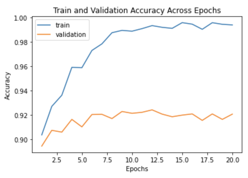
The network is trained on 90% of the entire training set, and the rest is held out for validation.
I trained the network for 20 epochs on a Tesla K80 GPU for 15 minutes. Notice that the validation accuracy curve begins to flatten after 8 epochs and fluctuates.
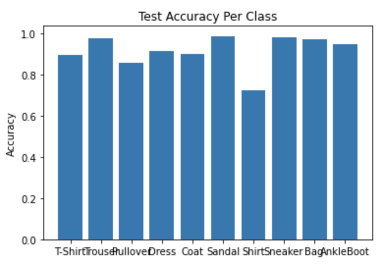
Here are the per class accuracies of the network for the test set. The hardest classes to classify are pullover and shirt.
| Class | Class Name | Test Accuracy |
|---|---|---|
| 0 | T-shirt/top | 89.6% |
| 1 | Trouser | 97.9% |
| 2 | Pullover | 86.2% |
| 3 | Dress | 91.4% |
| 4 | Coat | 90.3% |
| 5 | Sandal | 99.0% |
| 6 | Shirt | 76.3% |
| 7 | Sneaker | 98.4% |
| 8 | Bag | 97.6% |
| 9 | Ankle boot | 94.9% |
| Overall | 92.2% |
|
Here is a table showing some images that were classified correctly and some that weren't. The first column is the actual class name of the images in the middle, and the last column are the classes predicted by the model of the two incorrectly classified images.
| Class Name | Classified Correctly | Classified Incorrectly | Predicted Class Name | ||
|---|---|---|---|---|---|
| T-shirt/top |

|

|

|

|
Shirt, Shirt |
| Trouser |

|

|

|

|
Dress, Dress |
| Pullover |

|

|

|

|
Shirt, Shirt |
| Dress |

|

|

|

|
Shirt, Shirt |
| Coat |

|

|

|

|
Shirt, Shirt |
| Sandal |

|

|

|

|
Sneaker, Sneaker |
| Shirt |

|

|

|

|
T-shirt/top, Dress |
| Sneaker |

|

|

|

|
Sandal, Ankle boot |
| Bag |

|

|

|

|
T-shirt/top, Shirt |
| Ankle boot |

|

|

|

|
Sandal, Sneaker |
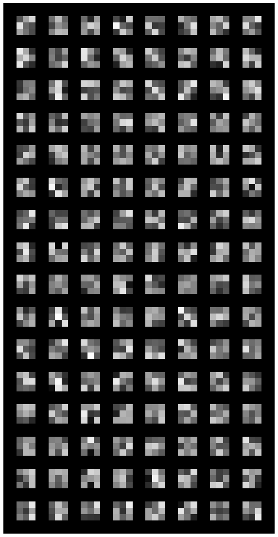
The first convolution layer has 128 3x3 filters. The learned filters are displayed below.
|
Part 2: Semantic Segmentation
Overview
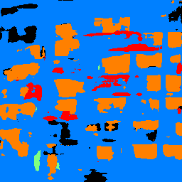
In this part, we use a CNN to do image segmentation, the task of classifying each pixel to the correct object class. We have used the Mini Facade dataset, which consists of images of different cities around the world and diverse architectural styles (in .jpg format), shown as the image on the left. It also contains semantic segmentation labels (in .png format) in 5 different classes: balcony, window, pillar, facade and others.
| Class | Class Color |
|---|---|
| Others | Black |
| Facade | Blue |
| Pillar | Green |
| Window | Orange |
| Balcony | Red |
Implementation Details
Overview: The network is built around an encoder-decoder scheme, where we have both up and downsampling of the image using convolutions and transposed convolutions. We trained the network for 50 epochs in batches of 16 samples using Tesla K80 GPU for 1 hour. Even though we do predict the network to perform better with further adjustments to the layer design (for example, by increasing number of downsampling and upsampling layers, which has shown to increase accuracy), these would require better GPUs or parallelization of GPUs, as more intricate networks require more CUDA memory.
We have also attempted using only 6 convolutional layers (4 downsampling convolutions, 1 convolution transpose and 1 final convolution), with far worse results, which we report in the results section. This followed similar layer design to below, where each convolution (kernel size of 3, padding of 1) was followed by a BatchNorm and a ReLU layer. Transposed convolutional layer has a kernel size of 2 and stride of 2. We also used cross-entropy loss as the prediction loss and the Adam Optimizer with a learning rate of 1e-3 and a weight decay of 1e-5, and trained for 50 epochs.
Layer Design: The network has 6 downsampling layers, 2 middle layers and 6 upsampling layers. Downsampling layers consist of one convolutional layer, BatchNorm Layer and a ReLU layer. Each convolutional layer has a kernel size of 3 and padding of 1. Upsampling layers consist of one transposed convolutional layer, one interpolation, and convolutional layer, BatchNorm layer and a ReLU layer. The transposed convolutional layer has a kernel size of 2 and stride of 2 and each convolutional layer has a kernel size of 3 and padding of 1. The intuition behind this design is that in the upsampling stages, we have convolutional layers to propagate information to higher resolution layers.
Loss and Optimizer: We used the cross-entropy loss as the prediction loss and the Adam Optimizer with a learning rate of 1e-3 and a weight decay of 1e-5.
Experiments Conducted: Initial experiments consisted of architecture designs. We have attempted using only convolution layers, using one final upsampling convolutional layer, including/excluding BatchNorm layer, including/excluding MaxPool layer. Among them, our preliminary results showed that current architecture works the best. We predict that adding more layers (e.g., downsampling and upsampling layers) would increase accuracy, as going from 4 to 6 downsampling/upsampling layers increased the accuracy by more than 10%, so further adjustments may increase accuracy, though it may be more prone to overfitting. Then, we used different learning rates (1e-5, 1e-3, 1e0) and weight decays (1e-5, 1e-3) before finding that this current set of hyperparameters works the best.
Final Network:
Network: input -> [conv -> batchnorm -> relu] (64, 64, 128, 128, 256, 256) ->
[conv (256, 256) -> batchnorm -> relu -> conv (512, 512) -> batchnorm -> relu] ->
[conv_t -> conv ->batchnorm -> relu -> conv ->batchnorm -> relu] -> outputs
Optimizer: Adam (lr=1e-3, weight_decay=1e-5)
Results
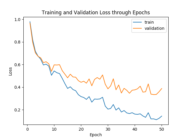
The network was trained on 80% of training data. Validation data was used for hyperparameter tuning. Below is a graph showing the training and validation losses across epochs:
|
We also use Average Precision (AP) on the test set to evaluate the learned model. The per class AP and overall AP are shown below.
| Class | Class Name | Average Precision |
|---|---|---|
| 0 | others | 0.736 |
| 1 | facade | 0.832 |
| 2 | pillar | 0.336 |
| 3 | window | 0.881 |
| 4 | balcony | 0.755 |
| Overall Average Precision | 0.708 | |
This is the per class AP and overall AP for using only 5 - 6 layers.
| Class | Class Name | Average Precision |
|---|---|---|
| 0 | others | 0.531 |
| 1 | facade | 0.702 |
| 2 | pillar | 0.112 |
| 3 | window | 0.789 |
| 4 | balcony | 0.362 |
| Overall Average Precision | 0.500 | |
My own Image: Here is an image I took of a building of a condominium (Reflections) in my neighboorhood in Singapore, which I have ran the segmentation on.
I am surprised by the results, as this photo is not aligned and in fact, leans to the side. However, all the images that were fed into the neural net were aligned. This shows that the classifier has not overfitted to the training set. Generally, however, the classifier is less successful in recognizing the balconies which show up in the same color and form (glass) as the windows.

|
|