Project 4: Classification and Segmentation

Yuhong Chen

Part 1: Image Classification

For the first part of this project, we'll be using convnets to perform image classification on the Fashion MNIST dataset.

Model Structure

I used a model with three convolutional layers with RELU activation and max pooling, followed by three fully connected layers to produce class probabilities for each class. Then I used binary cross-entropy loss with an Adam optimizer to optimize the network.

            nn.ReLU(inplace=True),
            nn.MaxPool2d(3, stride = 1), 
            
            nn.Conv2d(32, 32, kernel_size = 3), 
            nn.ReLU(inplace=True),
            nn.MaxPool2d(2, stride = 1),

            nn.Conv2d(32, 32, kernel_size = 3), 
            nn.ReLU(inplace=True),
            nn.MaxPool2d(2, stride = 1),
            
            Flatten(),
            
            nn.Linear(10368, 1024), 
            nn.ReLU(inplace=True),
            nn.Linear(1024, 128),
            nn.ReLU(inplace=True),
            nn.Linear(128, 10)

Training and Validation Accuracy

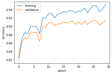
After training for 30 epochs, my model reached a test accuracy of 95.26%, and validation accuracy of 91.58%.

Per-Class Accuracies

I used the test set to generate a per-class accuracy for the network:

Class T-Shirt accuracy: 0.895
Class Trouser accuracy: 0.975
Class Pullover accuracy: 0.877
Class Dress accuracy: 0.923
Class Coat accuracy: 0.916
Class Sandal accuracy: 0.975
Class Shirt accuracy: 0.693
Class Sneaker accuracy: 0.986
Class Bag accuracy: 0.981
Class Ankle Boot accuracy: 0.937

The hardest class to classify was the Shirt, possibly because it had high similarity with the T-Shirt, whicl also had comparatively low accuracy. The Bag class had the highest accuracy, which makes sence as it's the only non-clothing class.

Samples Predictions

Class	Correct 1	Correct 2	Incorrect 1	Incorrect 2
T-Shirt
Trouser
Pullover
Dress
Coat
Sandal
Shirt
Sneaker
Bag
Ankle Boot

Filter Visualization

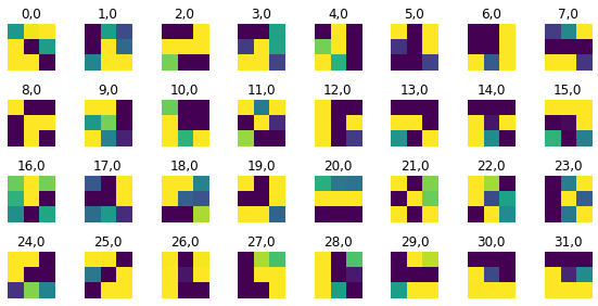
The weights of the kernels in the first layer are shown above. Most of them are simple features like slanted lines and corners.

Part 2: Semantic Segmentation

In the second part of this project, we use convnets for image segmentation, performed on the Mini Facade Dataset.

Model Structure

For this task, I use a fully convolutional/deconvolutional network, using only conv/deconv layers. This structure has the added benefit of being able to run on images of any size.

              nn.Conv2d(3, 8, kernel_size = 3, padding=1), 
            nn.ReLU(inplace=True),
            nn.Dropout2d(0.2),
            
            nn.Conv2d(8, 16, kernel_size = 3, padding=1), 
            nn.ReLU(inplace=True),
            nn.MaxPool2d(2, stride = 2),

            nn.Conv2d(16, 32, kernel_size = 3, padding=1), 
            nn.ReLU(inplace=True),
            nn.Dropout2d(0.2),

            nn.Conv2d(32, 32, kernel_size = 3, padding=1), 
            nn.ReLU(inplace=True),
            nn.Dropout2d(0.2),
          
            nn.Conv2d(32, 64, kernel_size = 3, padding=1), 
            nn.ReLU(inplace=True),
            nn.MaxPool2d(2, stride = 2), 

            nn.Conv2d(64, 64, kernel_size = 3, padding=1), 
            nn.ReLU(inplace=True), 

            nn.ConvTranspose2d(64, self.n_class, kernel_size=4, stride=4

I started with larger kernels and less layers, but found that using a deeper network with smaller kernels yielded better results.

Training and Validation Losses

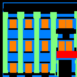
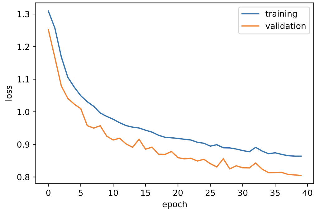
My model started with an average of 1.309 training loss and 1.25 validation loss. After 40 epochs, I had 0.864 training loss and 0.804 validation loss. My test set AP was 0.53457.

Sample Outputs

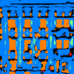
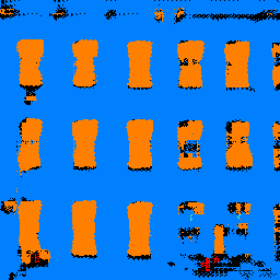
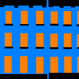
Input	Output	Ground Truth

My model did well on the windows and walls, which covered a large area, but relatively worse on baconies and pillars, which were somewhat rarer in the dataset. It makes sense that the model would prioritize learning the two most frequent classes in the dataset.