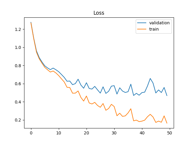
We plot the training accuracy and validation accuracy during training. Note that as training progresses, the network slowly overfits to the training set as the accuracy on the validation set no longer increases.
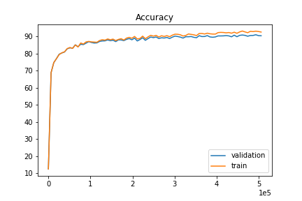
We use a network that has two convolution layer, each of which has 32 channels and kernel size of 3 and is follow the ReLU nonlinearity and a max-pooling layer of size 2. At the very end we have three fully-connected layers of size 120, 84, and 10 respectively. We use the cross-entropy loss and the network is trained with Adam with a learning rate of 0.001. 20% of the training set is used as validation set and the rest is used for training.
|
Accuracy by Classes
| Class Name | Accuracy (%) |
| T-shirt/top | 76.9 |
| Trouser | 97.1 |
| Pullover | 80.7 |
| Dress | 93.2 |
| Coat | 87.7 |
| Sandal | 98.1 |
| Shirt | 78.5 |
| Sneaker | 95.7 |
| Bag | 97.6 |
| Ankle boot | 96.5 |
As shown above, T-shirt is the hardest class to get probably due to its large variation. We also show 2 images from each class which the network classifies correctly and 2 more images which the network classifies incorrectly.
| Class Name | Classified Correctly | Classified Incorrectly |
| T-shirt/top |   |
  |
| Trouser |   |
  |
| Pullover |   |
  |
| Dress |   |
  |
| Coat |   |
  |
| Sandal |   |
  |
| Shirt |   |
  |
| Sneaker |   |
  |
| Bag |   |
  |
| Ankle boot |   |
  |
Below we visualize the learned filters by heat maps. We can see that some of the filters correspond to some interesting structures of the images in the training set.
| Layer | Filter Heatmap (32 each) |
| Conv1 |


 |
We use a network that has seven convolution layers, having 64, 128, 256, 512, 4096, 4096, 5 channels respectively and followed by the ReLU nonlinearity and two max-pooling layers of size 2. At the very end we have one tranposed convolution layer (though inaccurately a.k.a. deconvolution) for upsampling. We also use two drop-out masking layers before the We use the cross-entropy loss and the network is trained with Adam with a learning rate of 1e-3 and weight decay 1e-5.
 |
We are able to achieve an average precision (AP) of 0.64 on the test set.
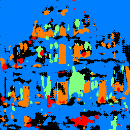
Below we also show a photo of a building that I took in Macau and the trained network's segmentation result from it. Note that the photo was taken at night and has different structure than those that are in the training set. From this photo we can see how well the network generalize to those that is not from the training data distribution. Note that it does relatively well on recognizing the windows (orange) but does poorly on recognizing the pillars (green) which is prevalent in the test image.
| Image | Segmentation |
 |
 |