CS194-26: Image Manipulation and Computational Photography Spring 2020
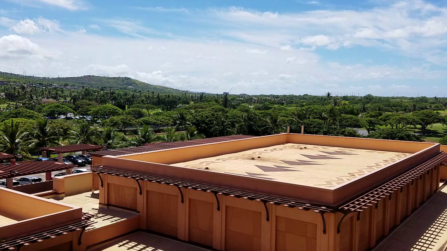
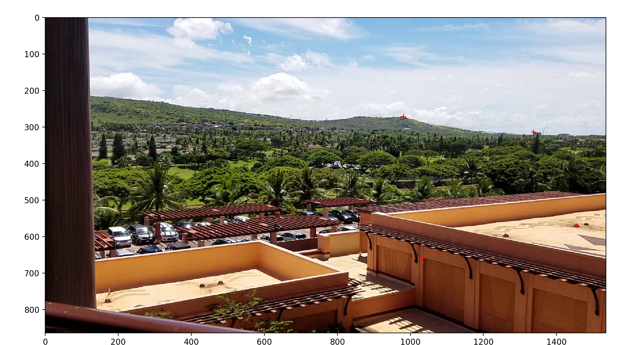
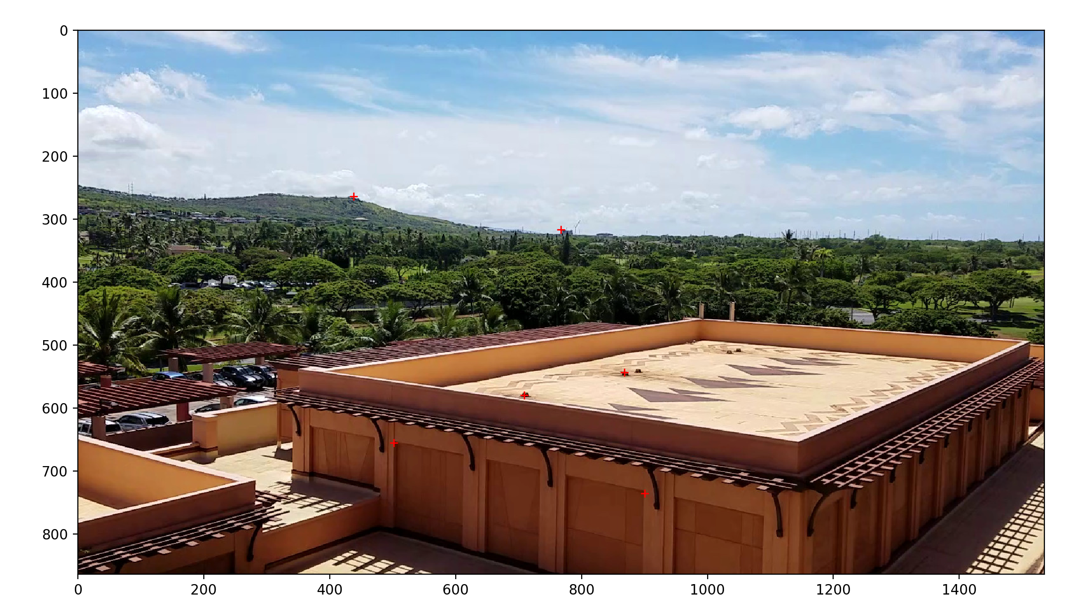
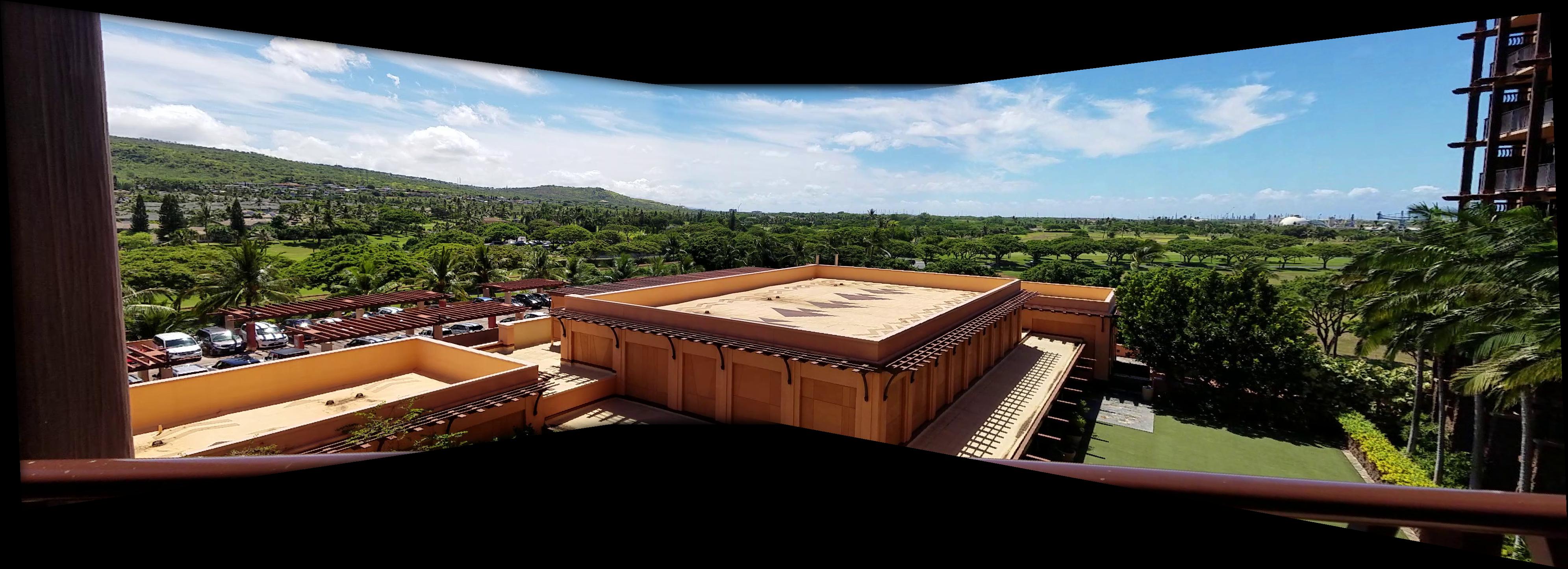
Here are some photographs that I took from the view of my hotel room in Oahu.
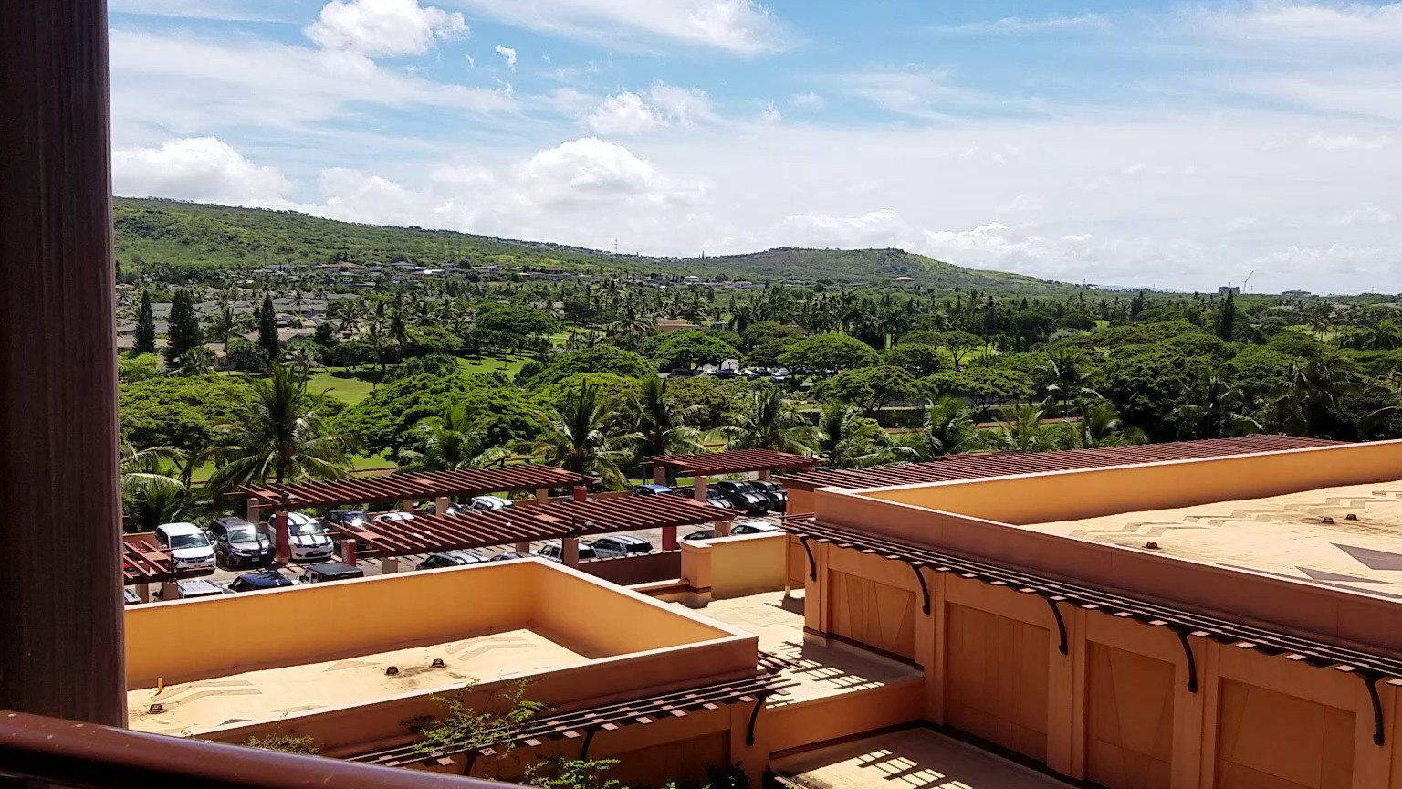
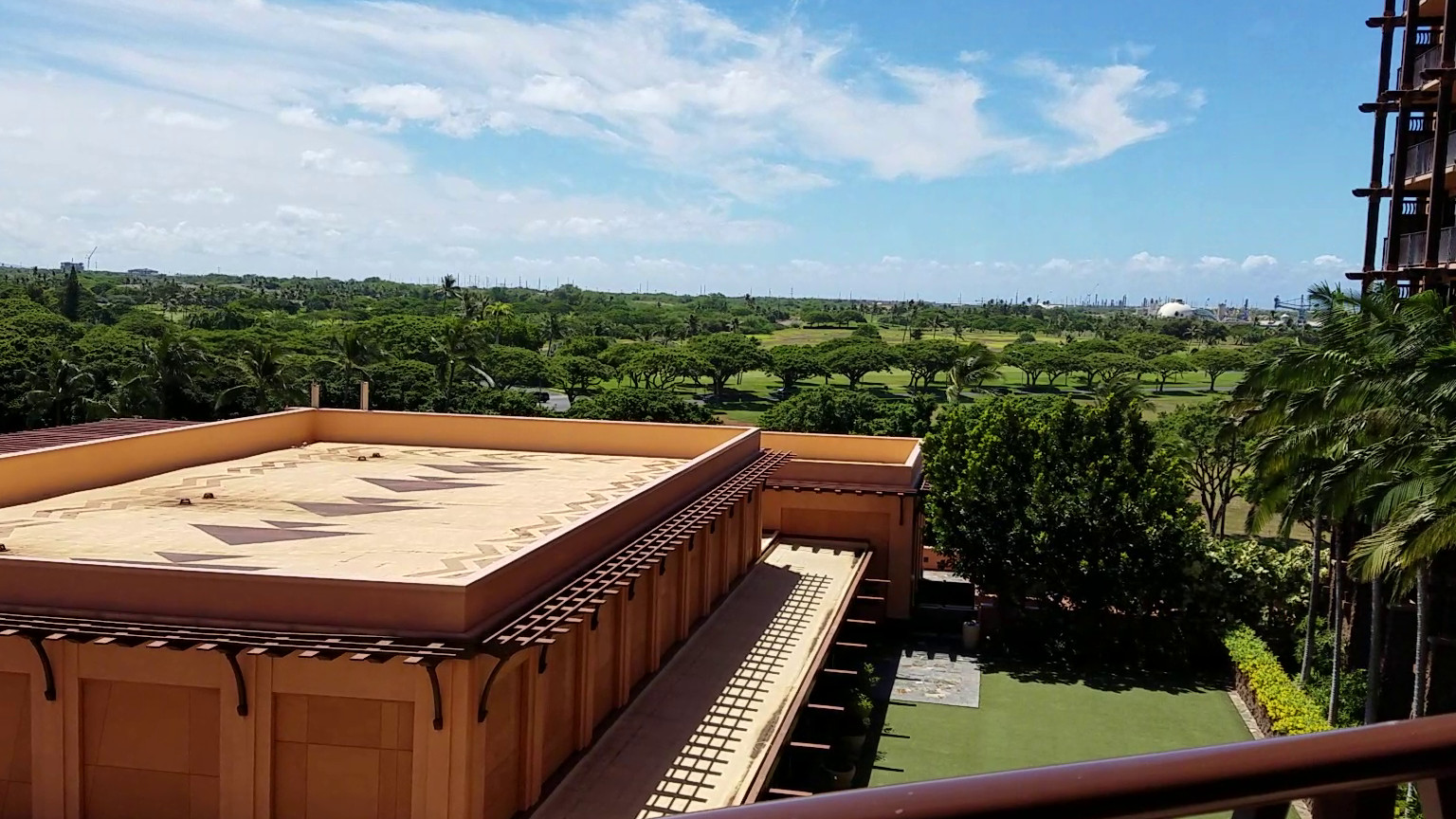
I chose these shots because the scenery is sufficiently far away that I can comfortably move the handheld camera while keeping it stationary enough.
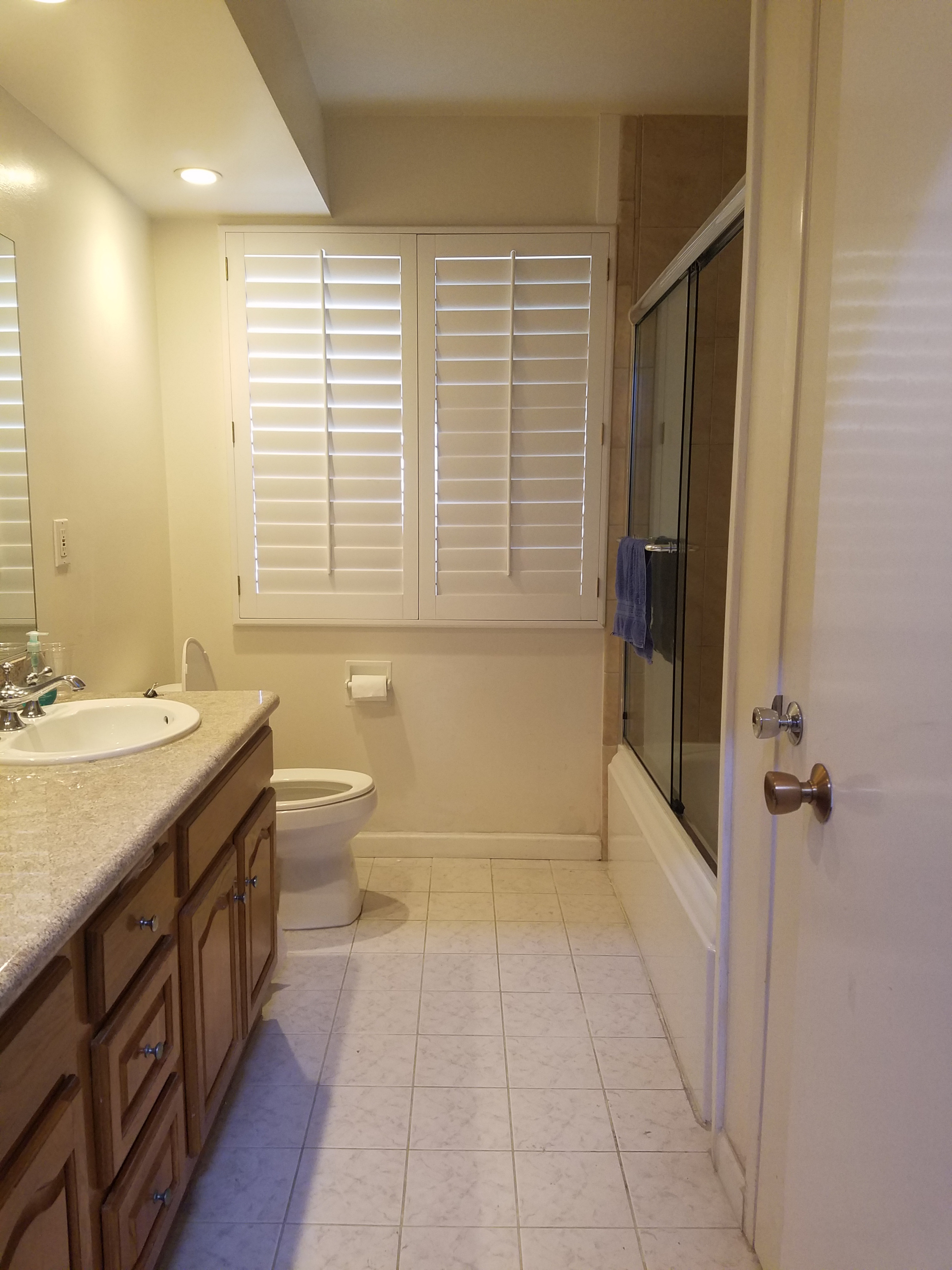
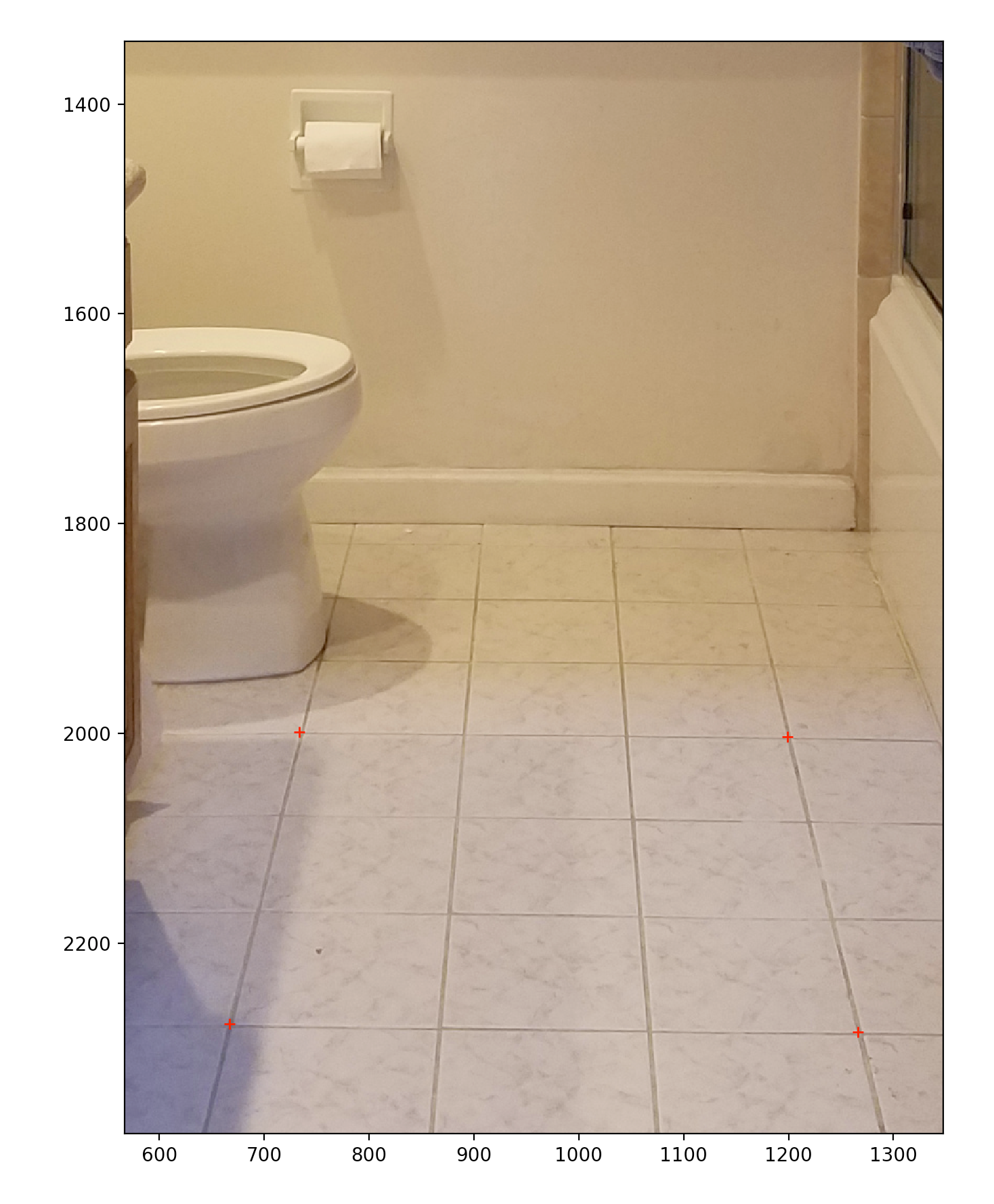
For rectification, I took a picture of my bathroom, and the provided facade image:
I implemented the function \(H\) as desired using matplotlib’s ginput. This allowed me to select correspondence points between two images like so:
We then use least-squares via the method described in lecture to solve for \(H\). See the bCourses code for implementation details.
We apply the solved-for homography to put the two images into the same perspective. This is done using inverse mapping. Each output pixel has its input location on the original image calculated, and then we sample appropriately to produce the final image:

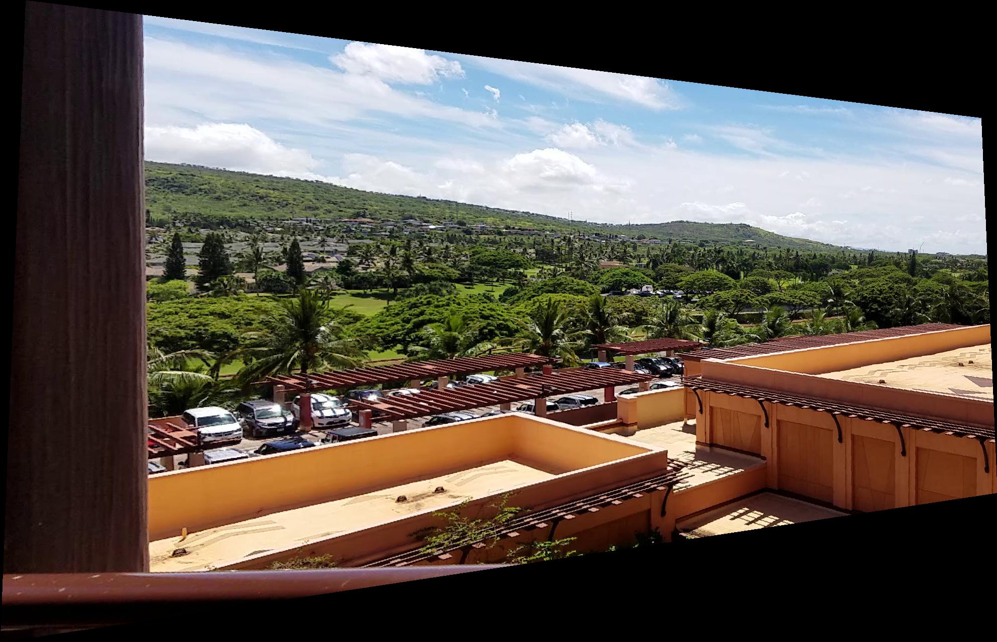
(Of course, the top image is identical since we used it to define the transform that all other images transform into.)
We can also apply the above procedure to rectify images. We select correspondence points like so:
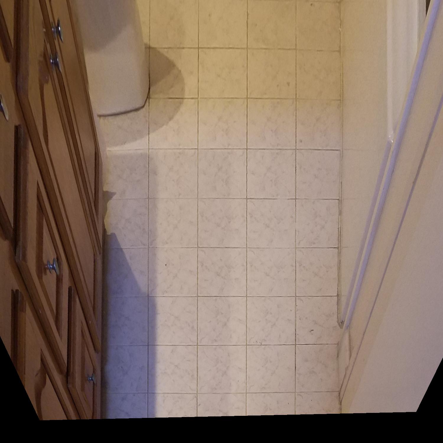
And then, we can compute the homography against a fixed grid to produce a rectified image:
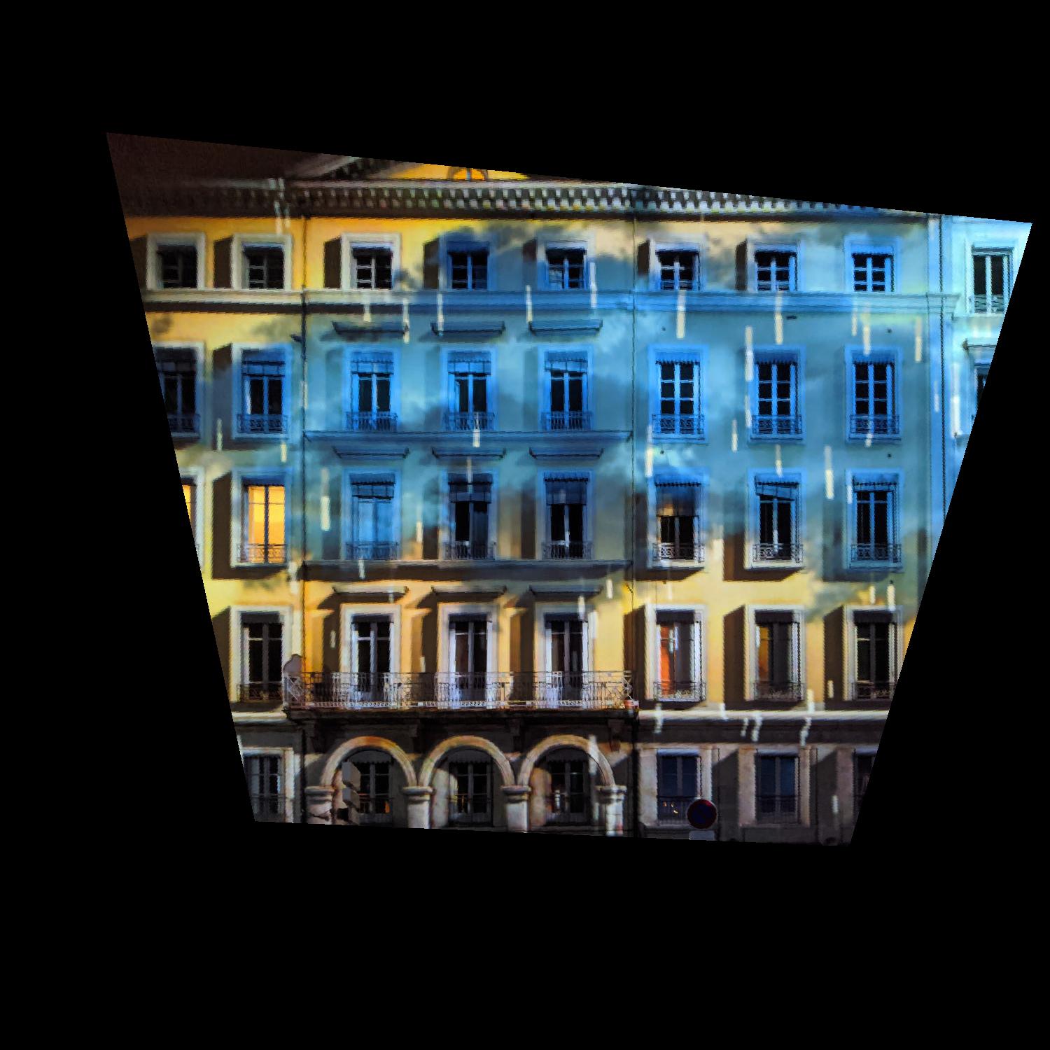
Repeated with the facade input:
We can use the technique described in lecture (distance from edge + feathered masking) to produce a clean blend between the warped Oahu images to produce a final mosaic. (Here I use all 3 images:)
The most interesting thing I learned was this new way to conceptualized photographs. Photographs are 2D projections of pieces cut out of a “pencil of rays” centered around the camera’s optic center. For this reason, we can actually recompute new camera angles or combine multiple photos together as in a mosaic. This technique is incredibly powerful, and demonstrates the general usefulness of a full homography transform in image processing.
HTML theme for pandoc found here: https://gist.github.com/killercup/5917178