import numpy as np
import matplotlib.pyplot as plt
%matplotlib inline
import skimage.io as skio
import skimage as sk
from glob import glob
from IPython.core.display import HTML
HTML("""
<style>
div.cell { /* Tunes the space between cells */
margin-top:1em;
margin-bottom:1em;
}
div.text_cell_render h1 { /* Main titles bigger, centered */
font-size: 2.2em;
line-height:0.9em;
}
div.text_cell_render h2 { /* Parts names nearer from text */
margin-bottom: -0.4em;
}
div.text_cell_render { /* Customize text cells */
font-family: 'Georgia';
font-size:1.2em;
line-height:1.4em;
padding-left:3em;
padding-right:3em;
}
.output_png {
display: table-cell;
text-align: center;
vertical-align: middle;
}
</style>
<script>
code_show=true;
function code_toggle() {
if (code_show){
$('div.input').hide();
} else {
$('div.input').show();
}
code_show = !code_show
}
$( document ).ready(code_toggle);
</script>
The raw code for this IPython notebook is by default hidden for easier reading.
To toggle on/off the raw code, click <a href="javascript:code_toggle()">here</a>.
""")
Part 1: Image Warping and Mosaicing
In this part of the project, we create homographies between images in order to warp one image to be in the perspective of the other. An homography is a 3x3 transformation matrix that transforms points from one coordinate system to another one coordinate system: p′=Hp. Then, we are able to stich and blend the warped pictures together to create a mosaic.
Recover Homographies
Because we're working with points of an image, our homography matrix will map a point p, $p = [x,y,1]^T$ in one image to $p' = w \cdot[x',y',1]^T$. We want to minimize the loss created by our homography: 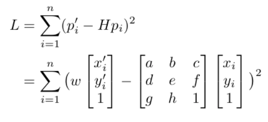
This equivalent to minimizing:
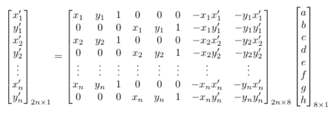
which we can formulate as a least squares problem: $Av=b$. If we solve for v that minimizes the error from the homography, we get an estimate of a,b,c,d,e,f,g,h.
Once we recover these values, we can warp the points in one image to another with the homography.
Warp the Images
In order to warp one image to another, I first calculated the bounds of the new image by piping the corners of the old image through the homography, calculating the bounde of the new image. After that, I used inverse warping to populate the new blank image with its corresponding points from the old image.
Image Rectification
We can make sure that our homography and warping are done correctly by rectifying an image, which is projecting an image onto another plane. To do this, you can compute a homography between an angled image and a flat rectangle, projecting that image onto the rectangle. You can see the results of rectifying two images from my apartment: a painting and the bathroom tiles.
fig=plt.figure(figsize=(20, 20))
columns = 2
rows = 2
images = ["monet.jpg","monet_rectified.jpg","bathroom.jpg","bathroom_rectified.jpg"]
for i in range(0, columns*rows):
fig.add_subplot(rows, columns, i+1)
plt.title(images[i].split(".")[0])
plt.axis('off')
skio.imshow(images[i])
plt.show()

Blend the images into a mosaic
In order to blend the images together, I first needed to define correspondences between the images. For each pair of images below, I identified between 13-26 points to align the images by. Then I warped one of the pictures to the persepective of the other. Lastly, I blended the pictures together. I created a canvas for each of the images, and aligned them with one of the correspondence points. The last step was to blend them together. From project 2, I found that a sigmoid applied to a linear increase from 0-1 in the section of the image requiring blending worked well, so I did the same thing.
fig=plt.figure(figsize=(40, 40))
columns = 3
rows = 3
images = ["room1.jpg","room2.jpg","room_blended.jpg","stonefire1.jpg","stonefire2.jpg","stonefire_blended.jpg","living1.jpg","living2.jpg","living_blended.jpg"]
for i in range(0, columns*rows):
fig.add_subplot(rows, columns, i+1)
plt.title(images[i].split(".")[0])
plt.axis('off')
skio.imshow(images[i])
plt.show()
