Part 1: Image Warping and Mosaicing
In this section, I took photos around my house to produce rectified images
and blended some into cool mosaics.
1.1 Recover Homographies
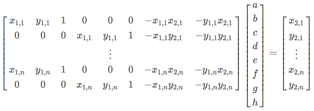
In order to warp my images, I recovered the 3x3 homography that relates the a pair of images.
I first used Python's ginput() function to pick 10 points on each pair of images. With the equation below,
I used least squares to recover [a, b, c, d, e, f, g, h] which would be the values in H (and i = 1).
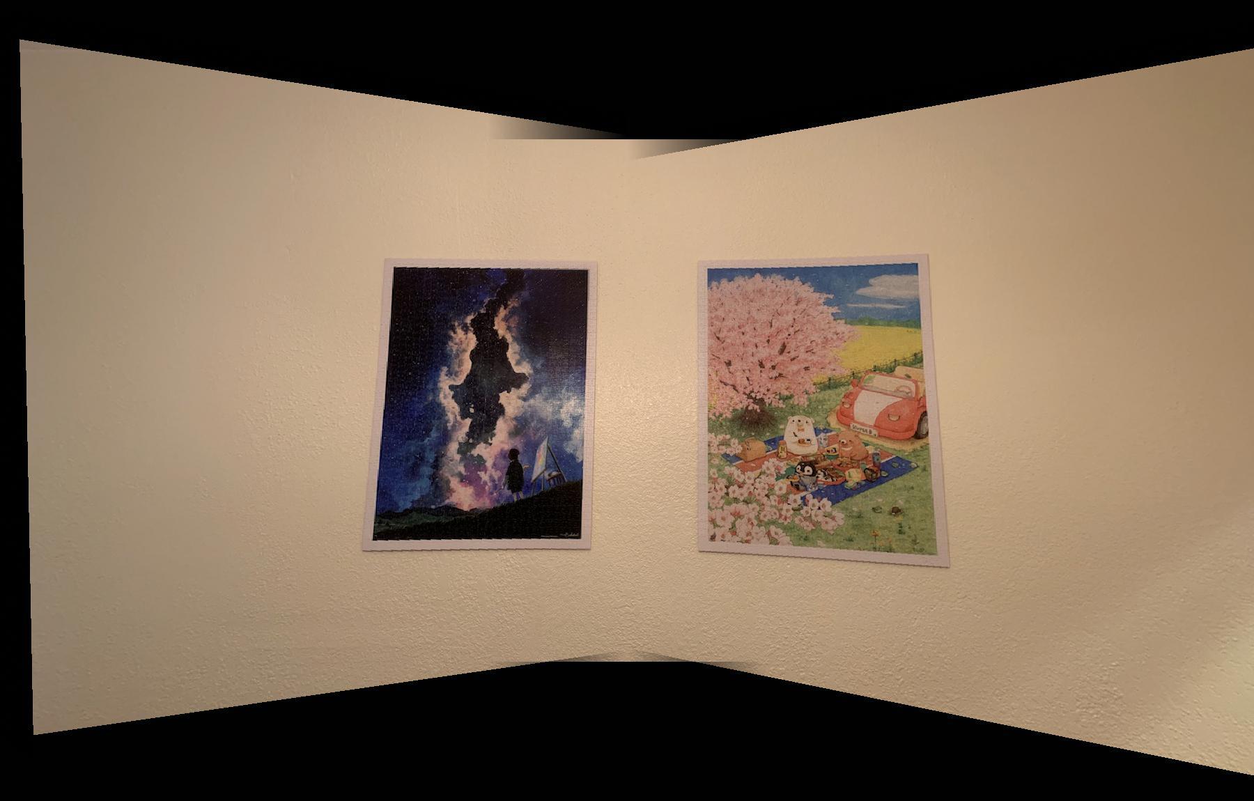
1.2 Image Warp and Rectification
Given the equation p' = Hp, I solved for p by applying the inverse homography matrix on the set of all
coordinates, then normalizing all the x,y coordinates to 1 by dividing by w. To prevent aliasing during
resampling, I applied linear interpolation so there wouldn't be any holes in the output. Below are some examples of
rectification. For these two specific images, I specified 4 points on the image, and 4 corners of a blank
destination image that would be used to reproduce H.
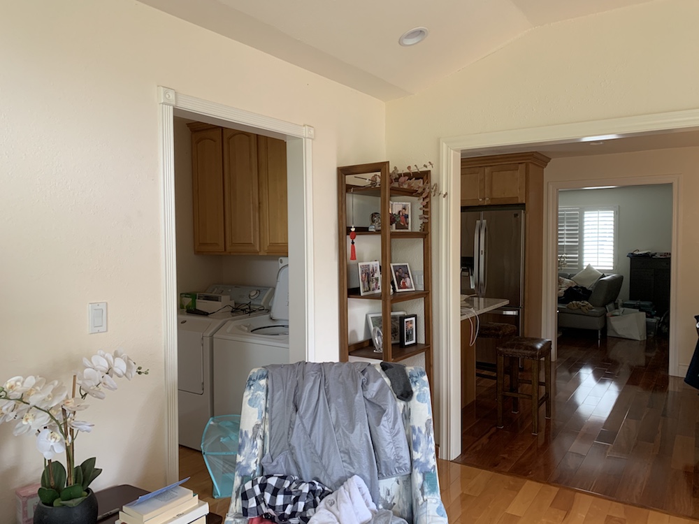
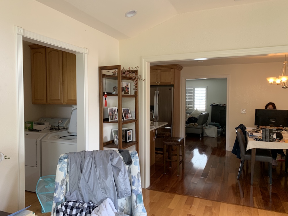
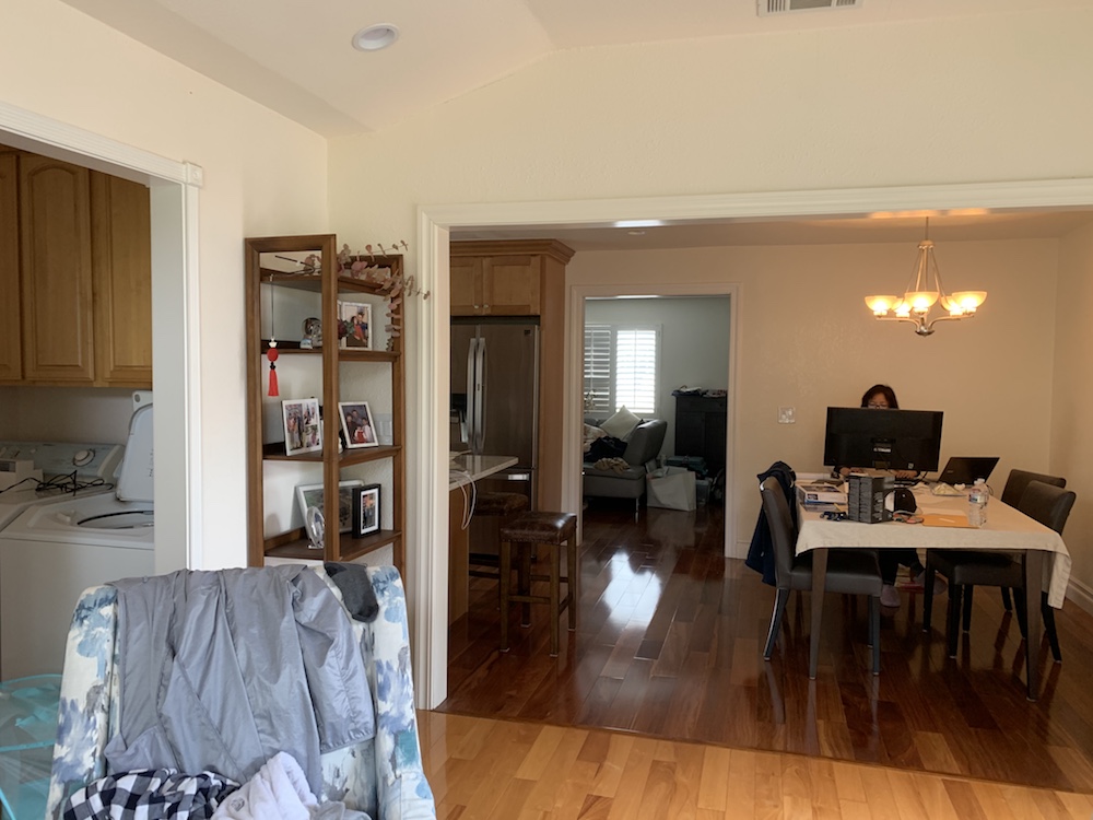
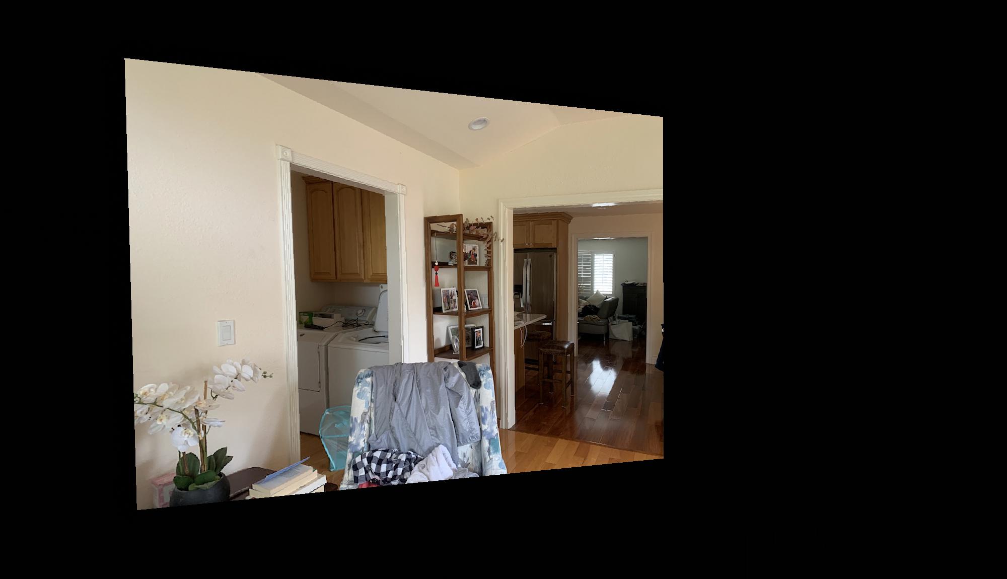
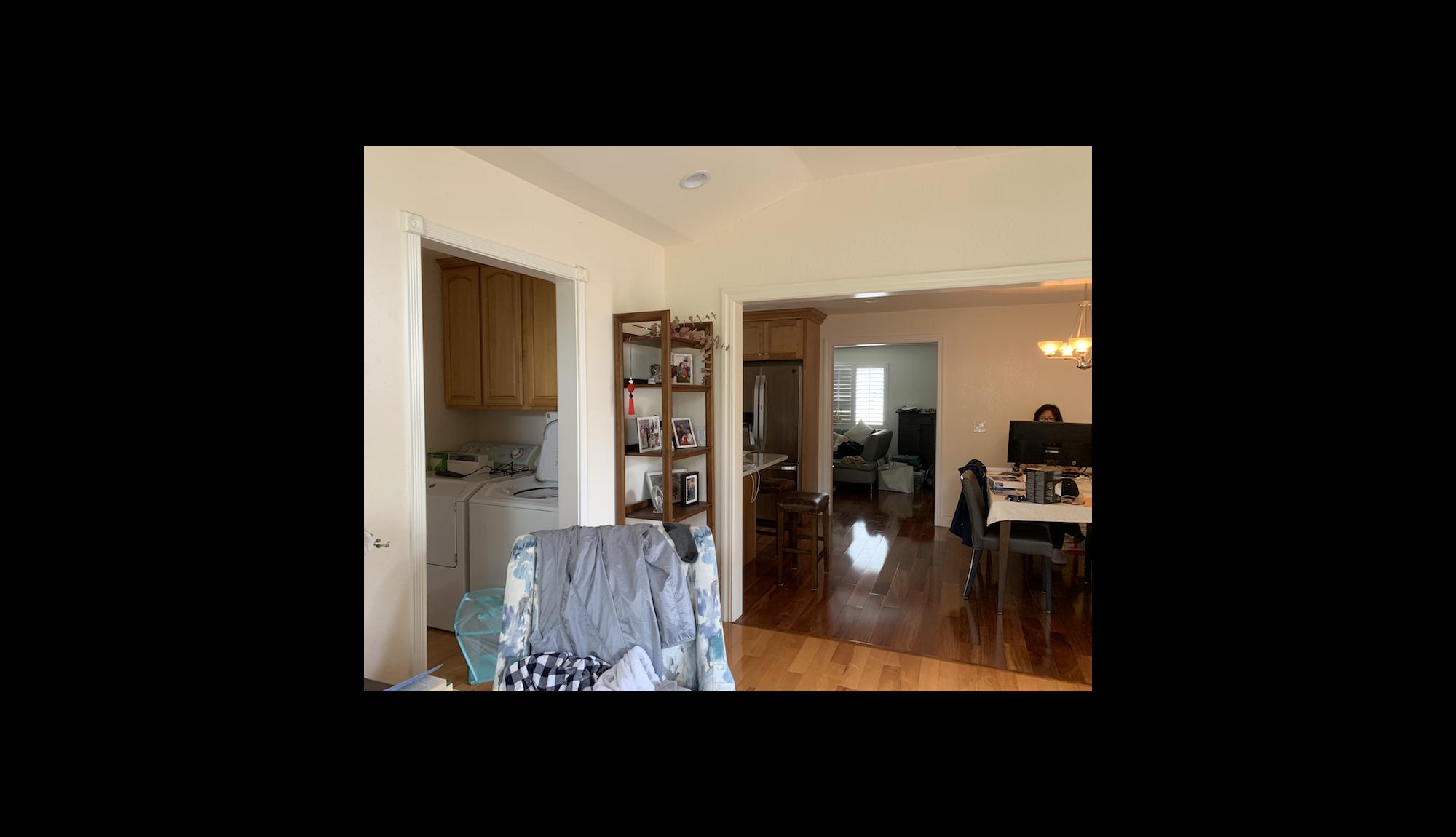
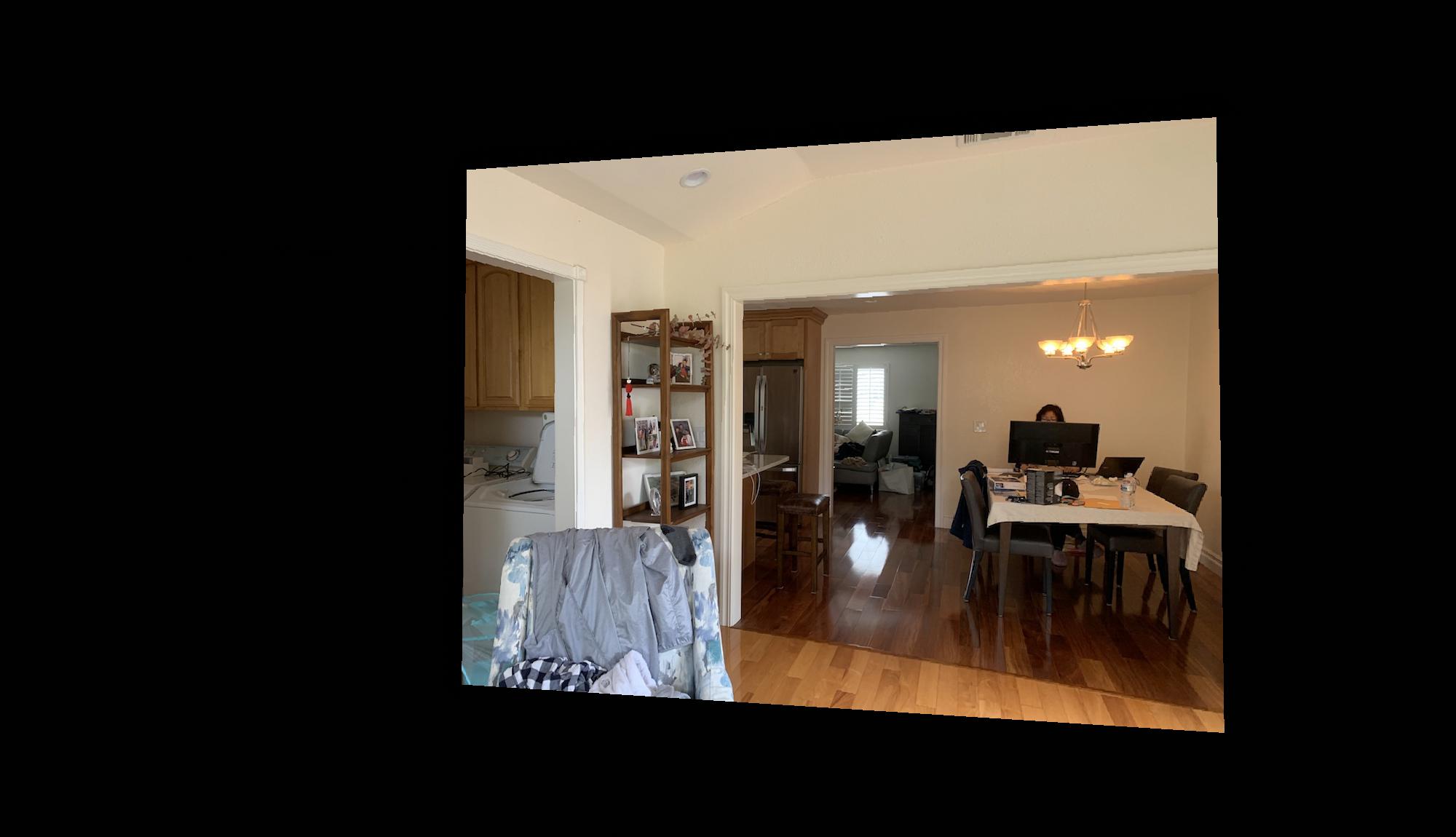
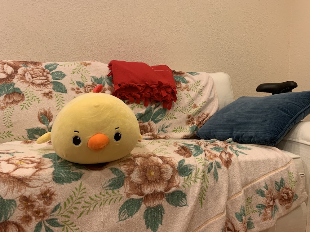
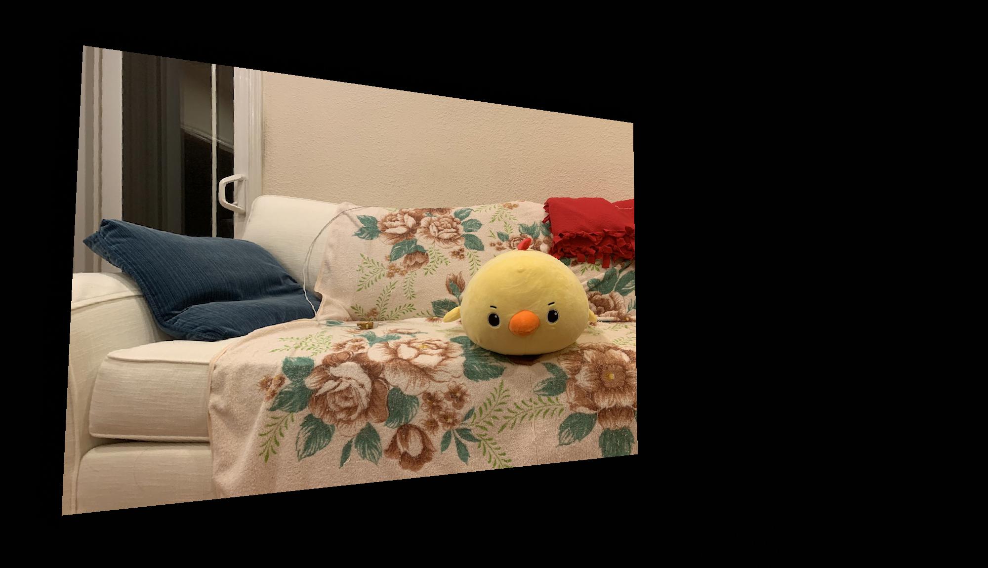
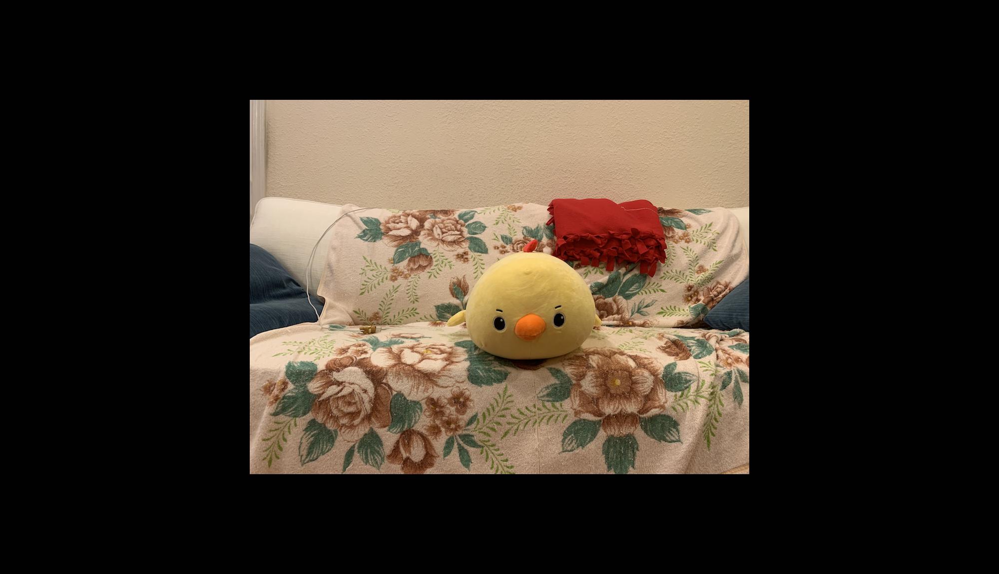
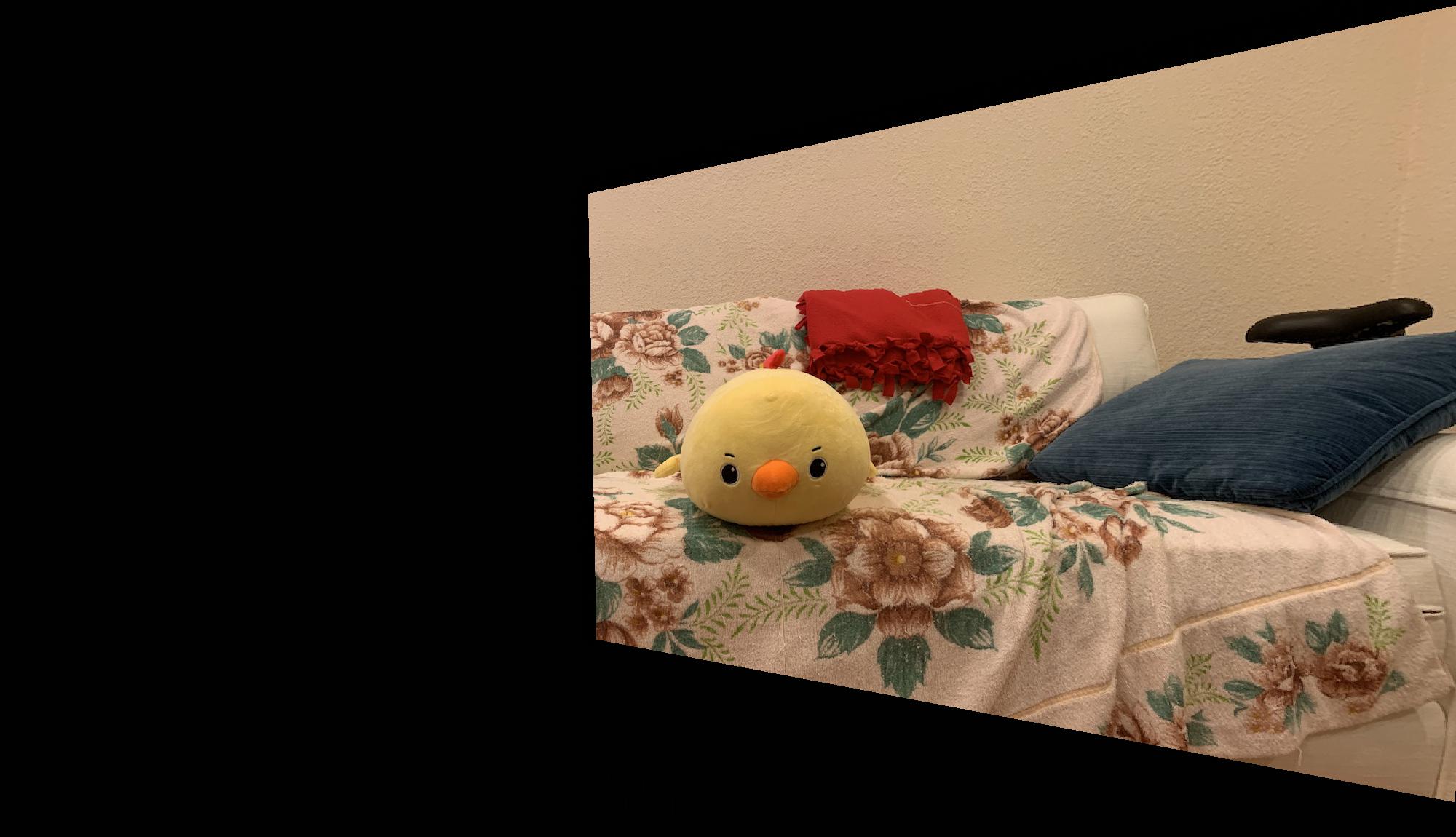
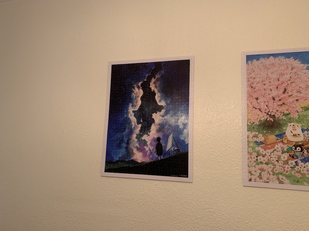
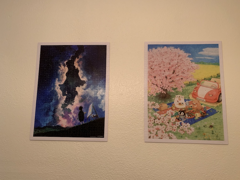
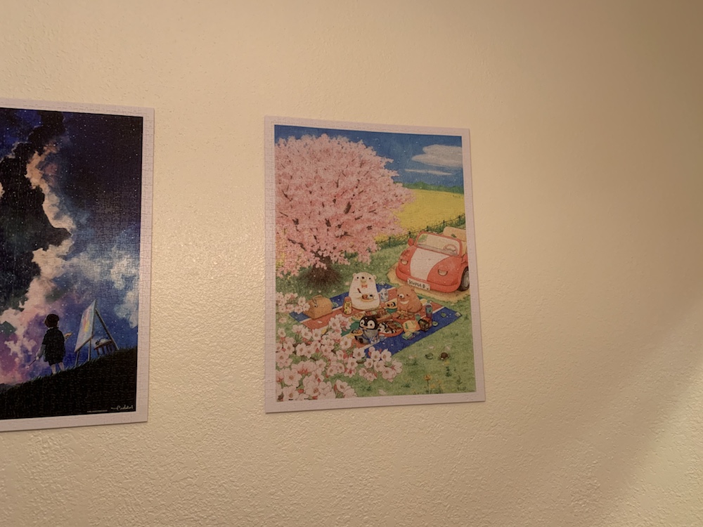
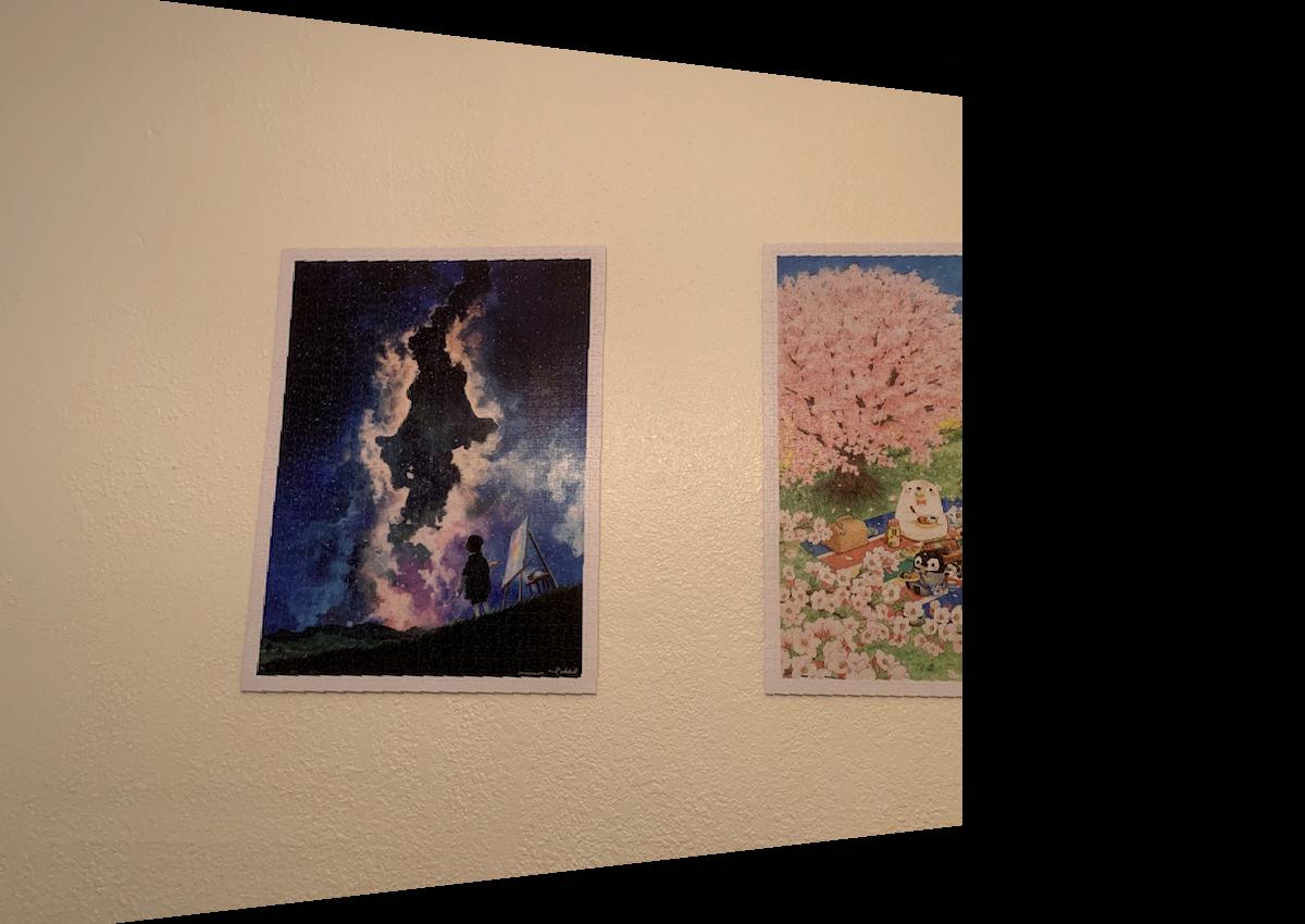
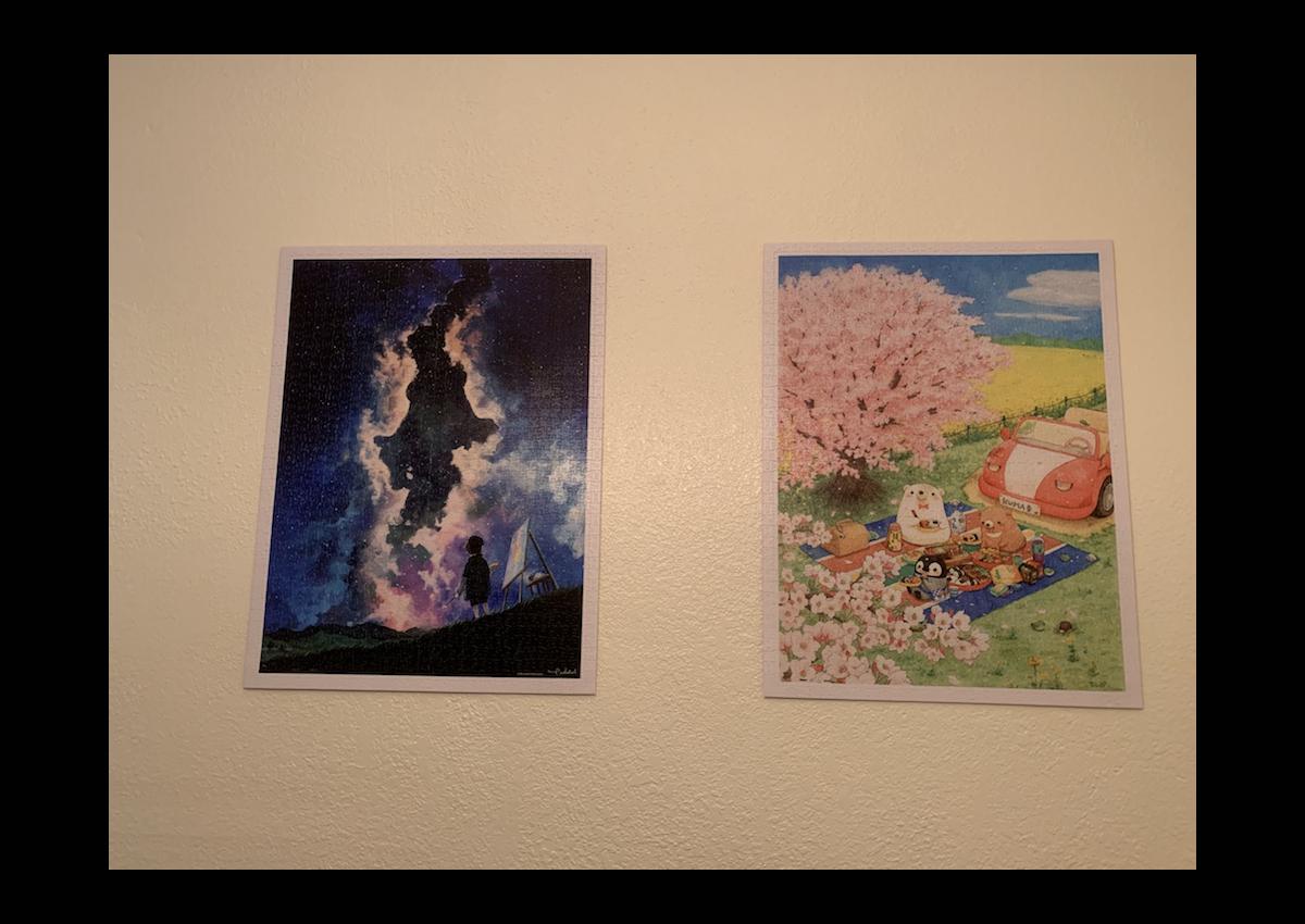
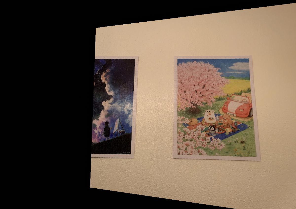
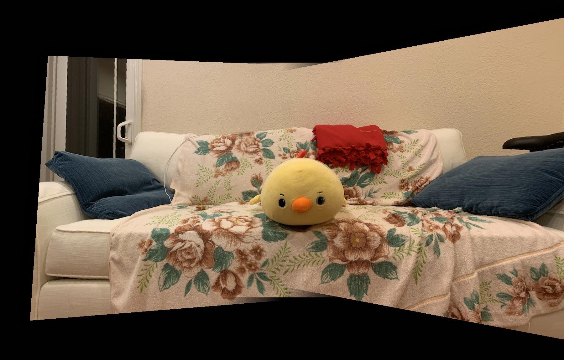
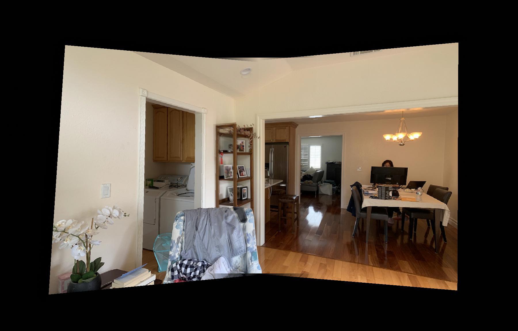
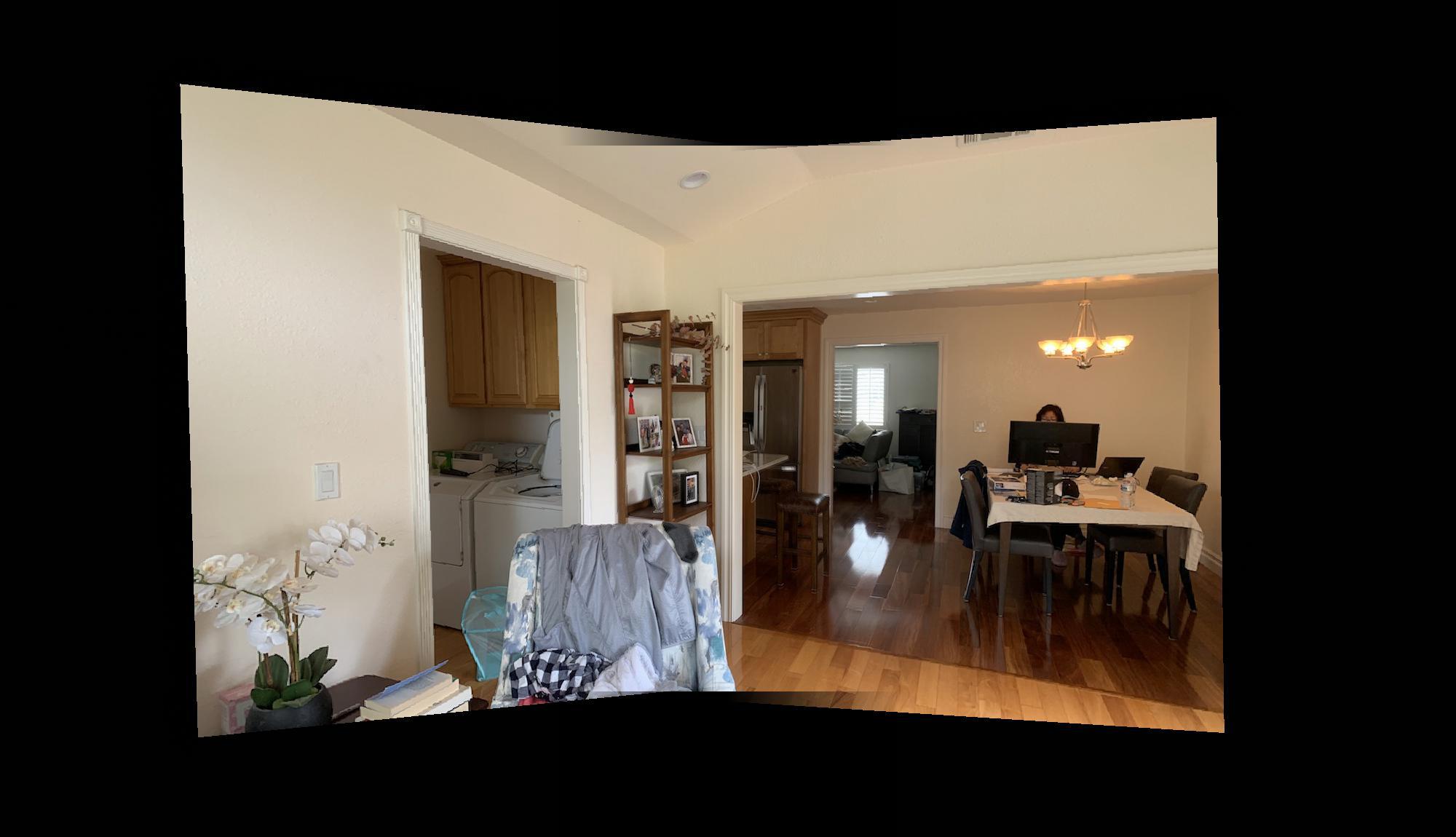
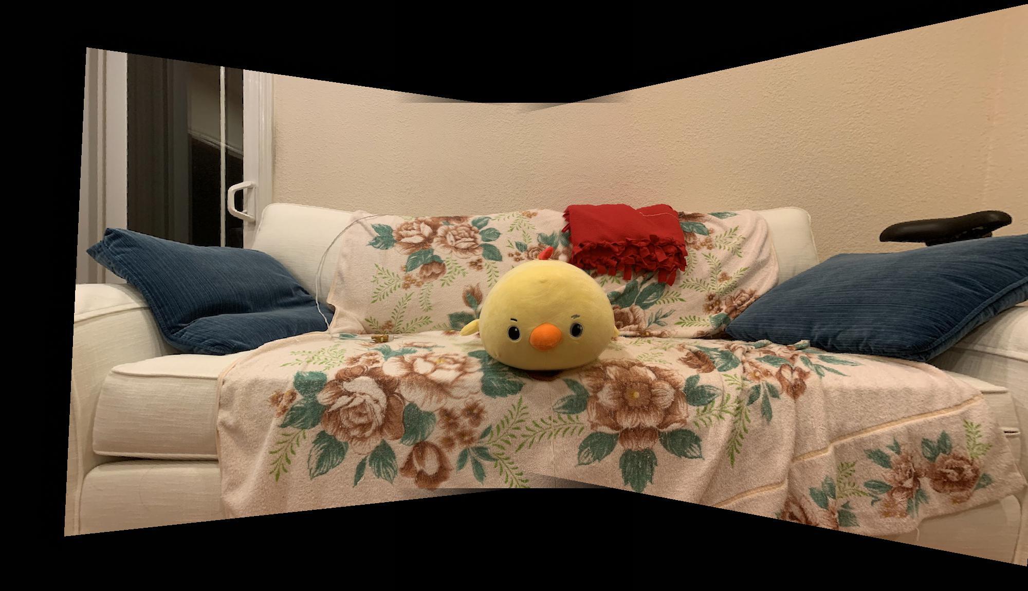
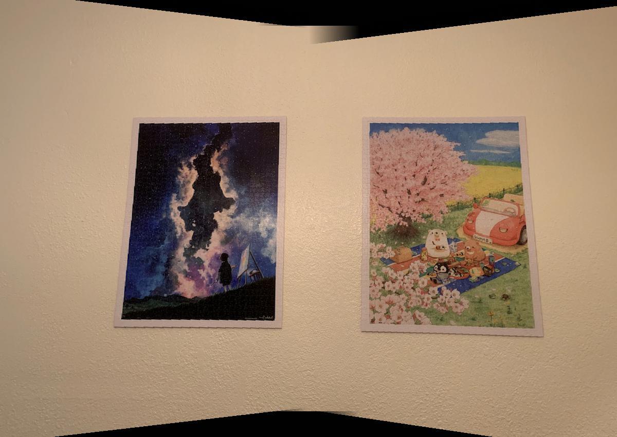
1.3 Image Stitching
For each panorama, I took 3 images (left, middle, right) and stitched them together to produce
one final result. I recovered the homography transformation from the left→middle images as well as
the transformation from right→middle images. I warped the left and right images to the middle image
using the method specified in the section above. Once I had all 3 images in their correct rectified form,
I played around with masks and applied alpha blending to each image.
1.4 Part 1 Takeaways
It was cool to see similar concepts from project 3 being applied to this project. I find it pretty
fascinating that the homography matrix does so much of the bulk of this transformation. Choosing the points
correspondances was quite tedious so I'm curious about the next part where we will automate that process.
Part 2: Feature Matching and Autostitching
In this section, I implemented a system as outlined in Brown's "Multi-Image Matching using Multi-Scale Oriented Patches".
Some methods I implemented include extracting feature descriptors, feature matching, and implementing RANSAC ot compute a homogrpahy.
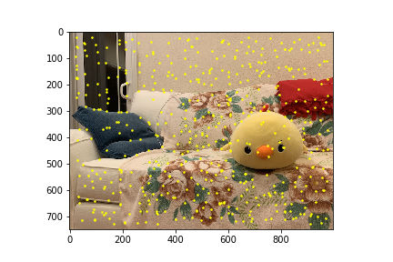
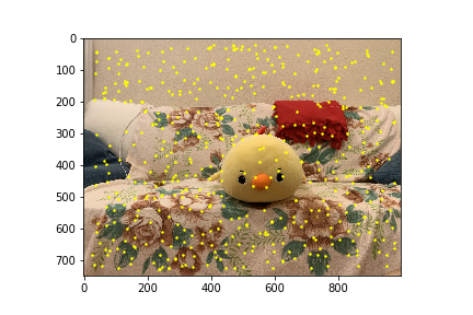
2.1 Detecting Corner Features and ANMS
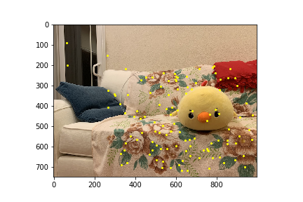
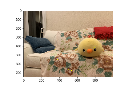
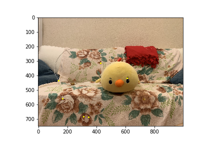
In order to generate many points of interest, I used the Harris Corner Detector to find the corners in my
images. I used the provided corner_harris and peak_local_max to generate these corners. There were far too many
points (16,000-19,000) that would show any significant result overlayed over the image so I will not provide an image
with all the harris corners overlayed.
Given the thousands of harris corners, I narrowed down the number of points by applying Adaptive Non-Maximal Suppression (ANMS). ANMS selects
the top 500 points with the largest minimum suppression radius. Below are the 500 points I get from applying ANMS.
2.2 Feature Descriptor Extraction
With our narrowed down 500 points, I extracted a 40x40 patch centered around each point and
downsampled this patch to size 8x8. Each patch is also normalised to a mean of 0 and a standard
deviation of 1. This allows the features invariant to affine changes in intensity.
2.3 Feature Matching
I vectorized the descriptors of all points and computed the squared distance from each feature in
the first image to each feature in the second image. I then applied the Lowe ratio test to find pairs
of points that seemed to be a match. The test takes the ratio of the SSD to the 1-NN to the SSD of the 2-NN
and sees if it's below a certain threshold that I defined as 0.1.
2.4 RANSAC
To narrow down the points even further so that we don't have any outliers, as outliers heavily affect
the homography calculation during least squares, we apply RANSAC. At each loop in RANSAC, I randomly sampled
4 points and computed the homography H from those randomly selected points. I used H to warp the points in the first image
to the points p' in the second image. I then computed the SSD error between p' and the real corresponding points in the second image.
If the SSD was below a threshold (0.05), I kept track points if the size of the set was currently the largest. After 1000
iterations, I used the resulting largest set of points as my point correspondances in calculating H.
2.5 Autostitching results
Since I could now compute H with the points derived from RANSAC, I could warp and stitch my
panorama the same way I did as part A. There doesn't seem to be a big difference between the
two results!
| Manual Stitching |
Auto Stitching |
|
|
|
|
|
|
|
|
|
2.6 Part 2 Takeaways
I'm continually amazed by how 'easy' it is to apply these algorithms to produce a seemlessly
accurate results! I've never really taken a course where I could see how a program could match
identical points between two images so it was really cool we had the opportunity to do that in
this project. Auto stitching definitely saved time and stress on my end because I was glad I didn't
have to select the points myself!