[Auto]Stitching Photo Mosaics
CS194-26 Spring 2020
Kamyar Salahi

Overview

In this project we will be stitching together images and exploring methods of creating homographies and determining correspondence points between images.
In the first part, we will manually define correspondences and warp them into composites. We will also be exploring rectification of images.
In the second part, we will automate this process and generate panoramas automatically. This algorithm utilizes Harris Corners, ANMS, Rotationally-Invariant Feature Descriptors, and RANSAC in order to generate an accurate homography mapping between the two image perspectives.

Part 1: Manual Correspondences, Warps, and Rectification

Introduction

A panorama is a “an unbroken view of the whole region surrounding an observer.” Traditionally, panoramas are created by taking a series of photos that have some overlap. These photos are subsequently aligned according to the features in these overlaps and stitched according to one of several models (spherical, cylindrical, and perspective). In this project, we will be using perspective projection. However, in many cases spherical or cylindrical projections can be more robust.

We will generate these panoramas by taking a series of photographs and rotating them as to have overlapping sections. We will then manually define correspondences and utilize Least Squares to recover the homography mapping of one image onto the other. We can then warp these images accordingly and then stitch the images together. In this implementation, multi-resolution blending is also utilized to generate more appealing results.

Homographies

Homographies are defined by a 3x3 matrix with 8 degrees of freedom.

$H = \begin{bmatrix} a & b & c \\ d & e & f \\ g & h & 1 \end{bmatrix}$

As a result of the eight degrees of freedom, a minimum of 4 points will be required to determine the homography. (One note here: the 4 points have to form a convex shape, otherwise the homography matrix cannot be uniquely determined.)

Our approach, however, will not utilize a simple inverse to recover the homography since our correspondence points are prone to noise and error. Consequently, we will utilize Least Squares to this end.

$\begin{bmatrix} x_{1,1} & y_{1,1} & 1 & 0 & 0 & 0 & -x_{1,1} x_{2,1} & -y_{1,1} x_{2,1} \\ 0 & 0 & 0 & x_{1,1} & y_{1,1} & 1 & -x_{1,1} y_{2,1} & -y_{1,1} y_{2,1} \\ & & & & \vdots & & & \\ x_{1,n} & y_{1,n} & 1 & 0 & 0 & 0 & -x_{1,n} x_{2,n} & -y_{1,n} x_{2,n} \\ 0 & 0 & 0 & x_{1,n} & y_{1,n} & 1 & -x_{1,n} y_{2,n} & -y_{1,n} y_{2,n} \\ \end{bmatrix} \begin{bmatrix} a \\ b \\ c \\ d \\ e \\ f \\ g \\ h \end{bmatrix} \begin{bmatrix} x_{2,1} \\ y_{2,1} \\ \vdots \\ x_{2,n} \\ y_{2,n} \end{bmatrix}$

We can now use multiple correspondence points to recover the homography. For manual selection, I used roughly 10 correspondence points between images.

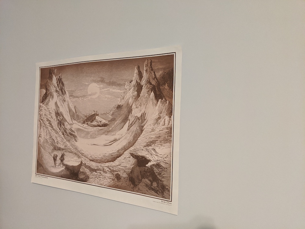
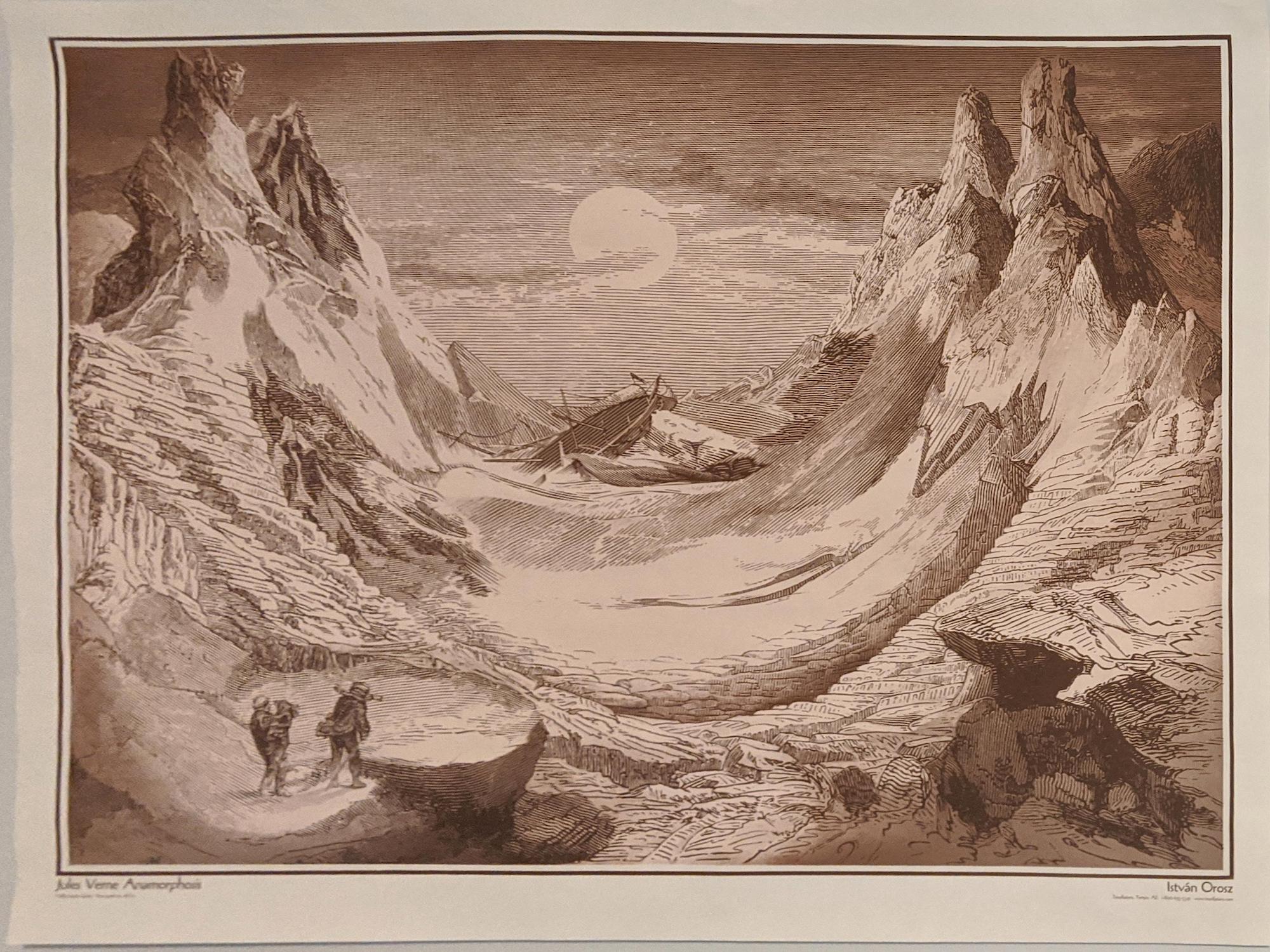
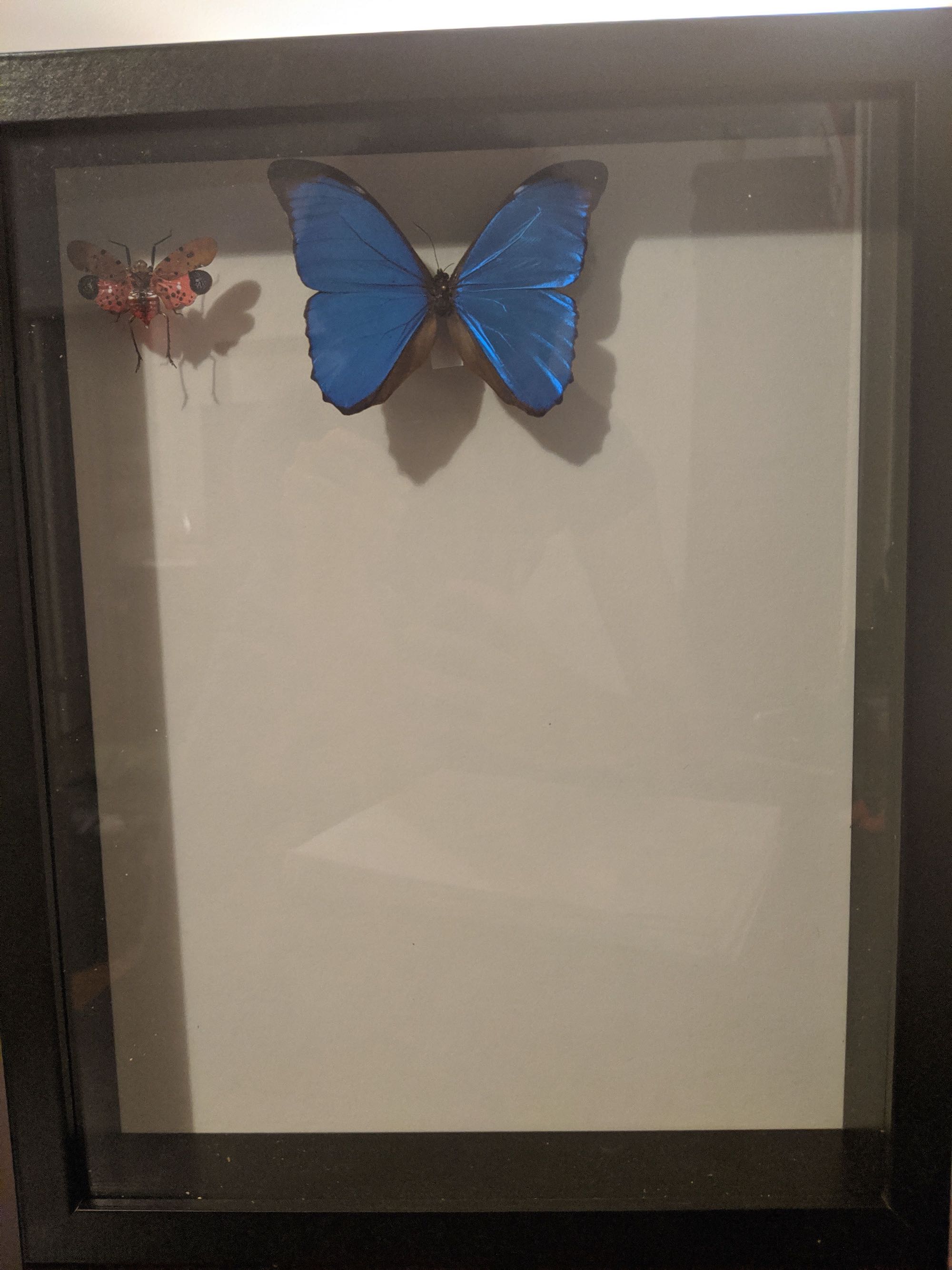
Image Rectification

Given that we have figured out how to find homographies, it is now possible to perform an inverse warp. This is performed by multiplying every point in the output image by the inverse of the homography matrix to recover the corresponding point on the origin image. We can select four correspondence points on the rectangle’s corners and map them to any given dimension. Bicubic interpolation was utilized here as to minimizing aliasing artifacts.

Istvan Orosz Poster

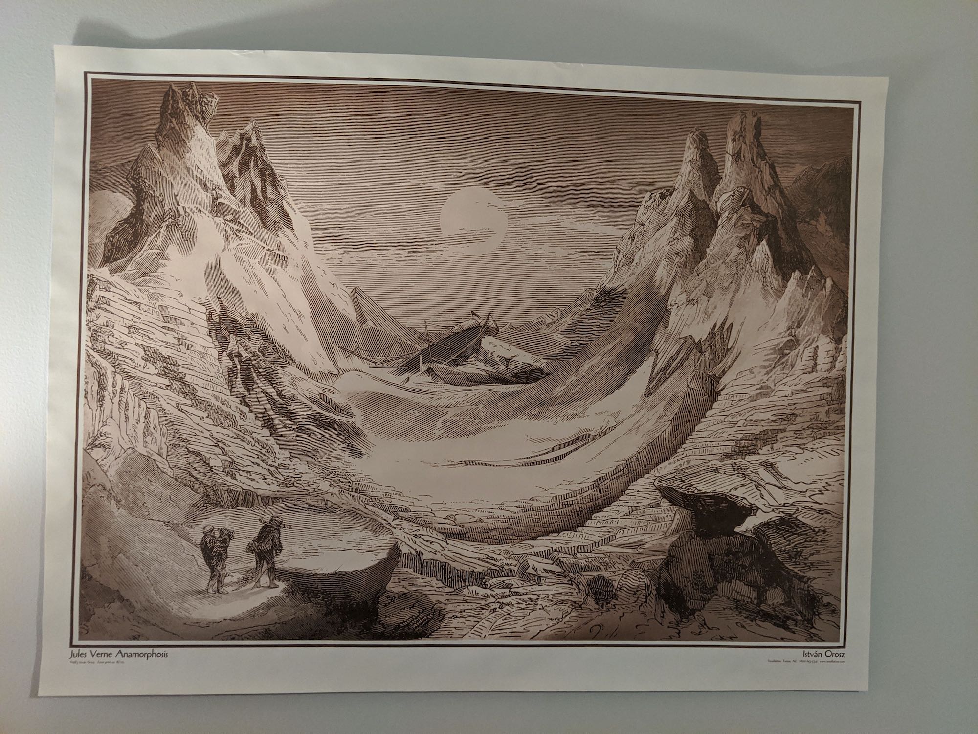
Aliasing (without bicubic interpolation)

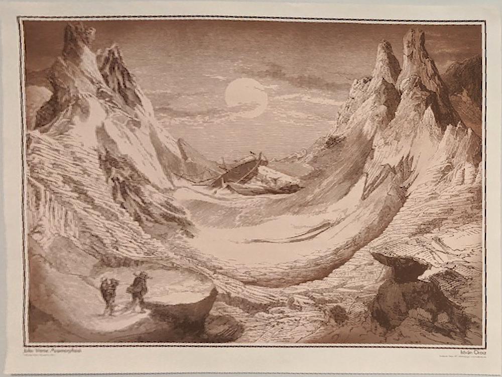
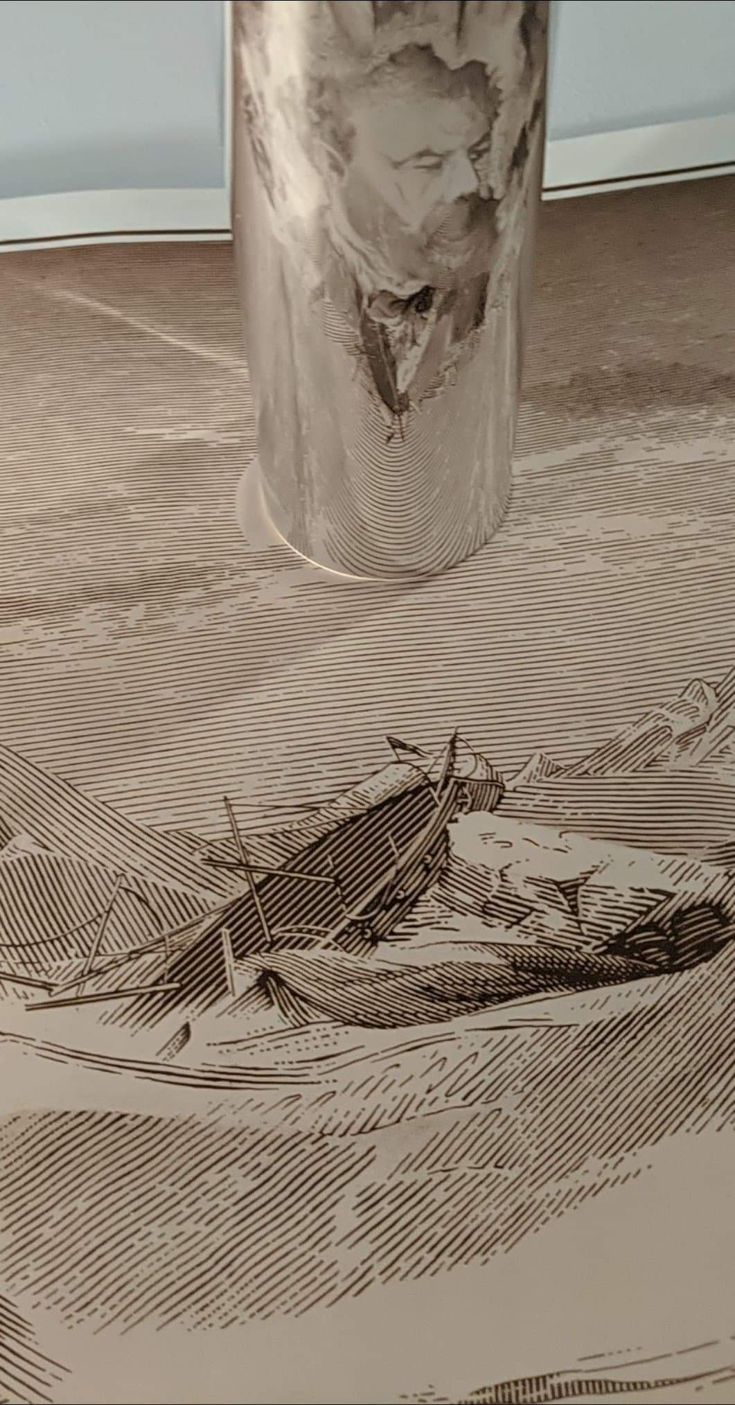
Anamorphic Art

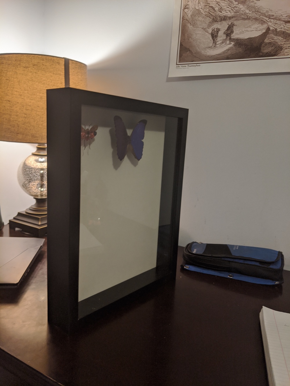
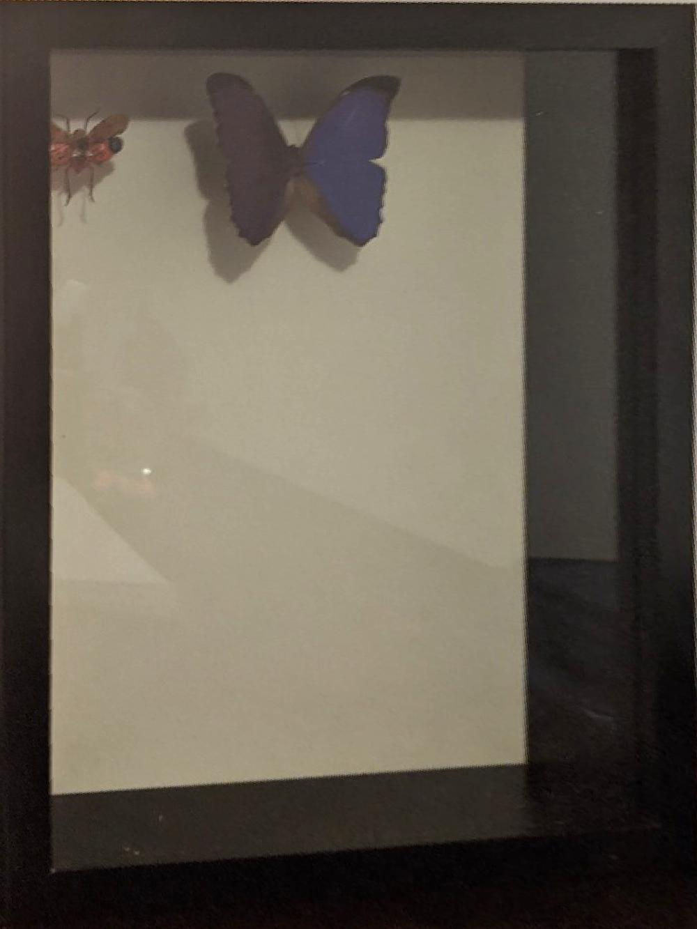
Butterfly Shadow Box

Mosaics

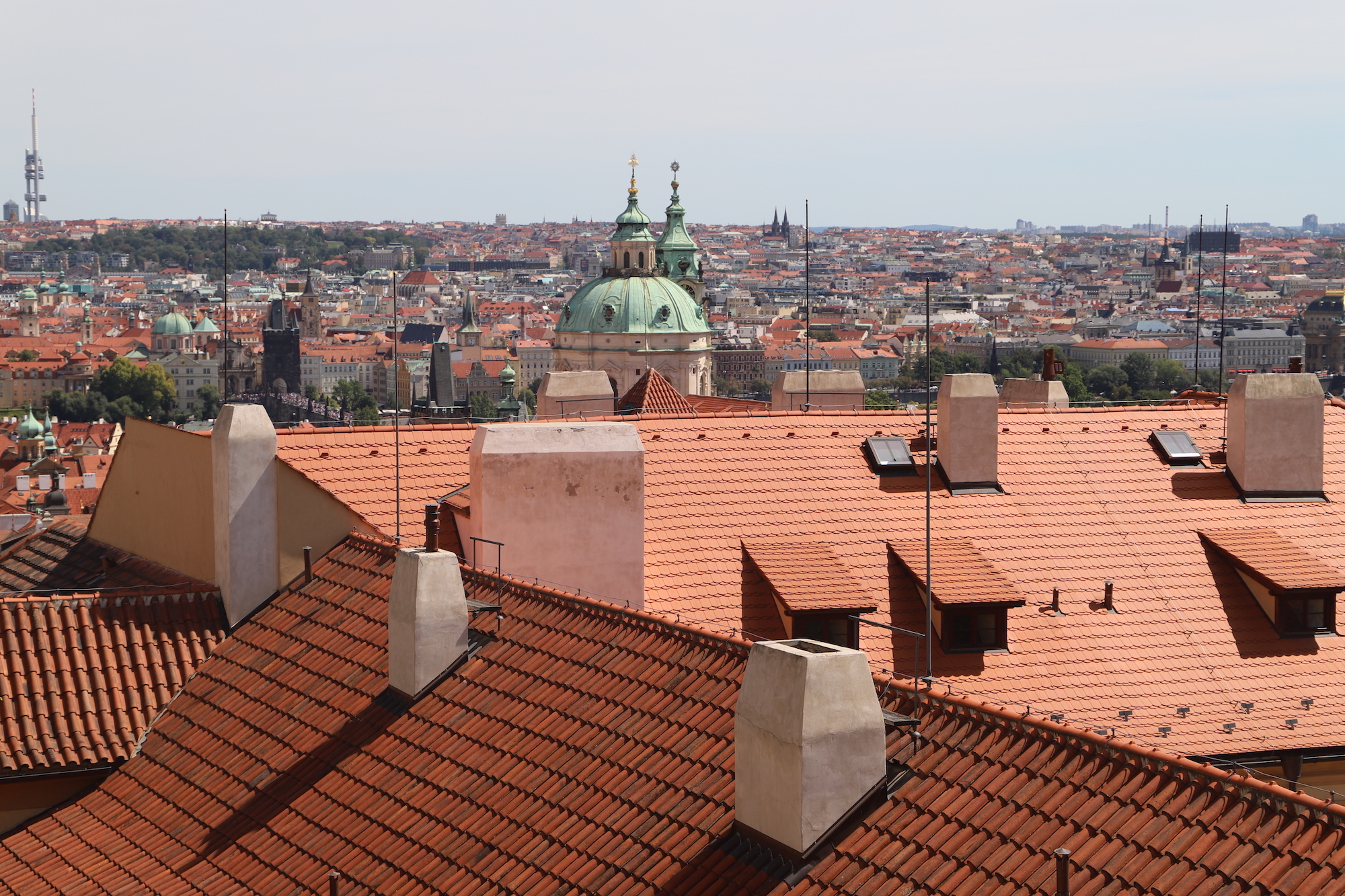
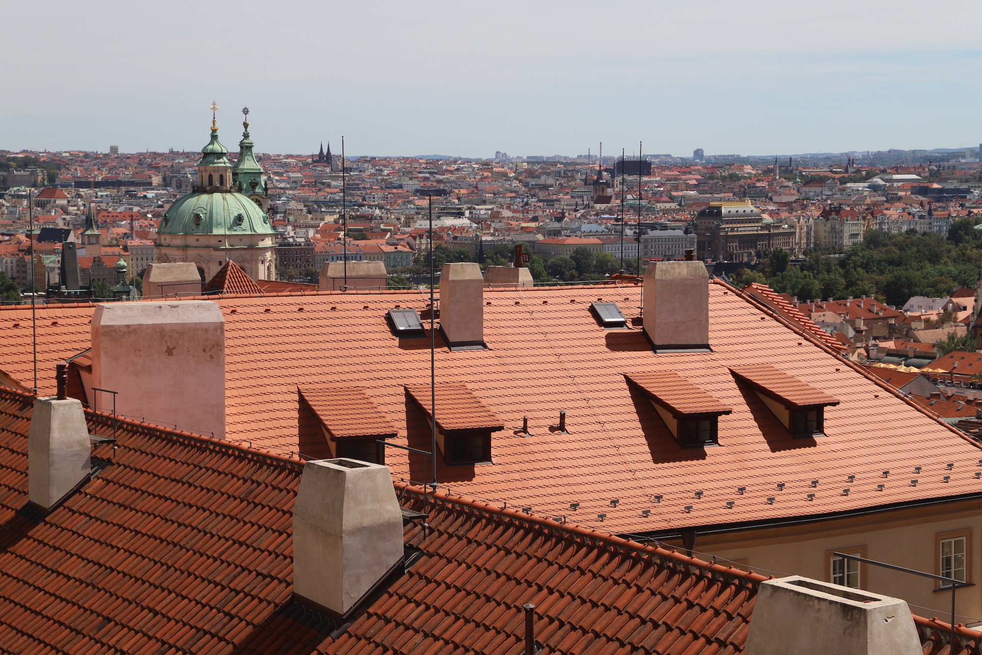
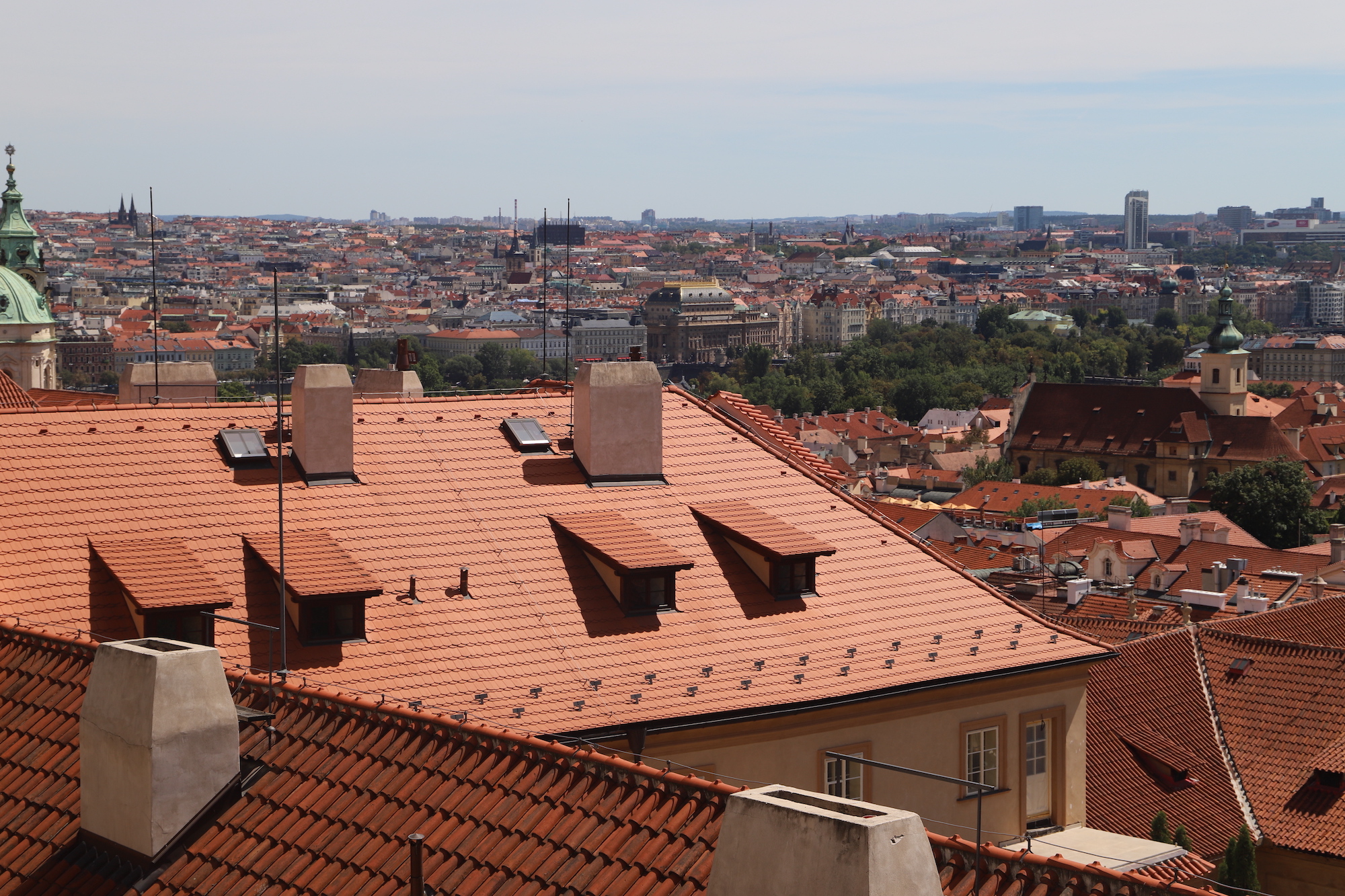
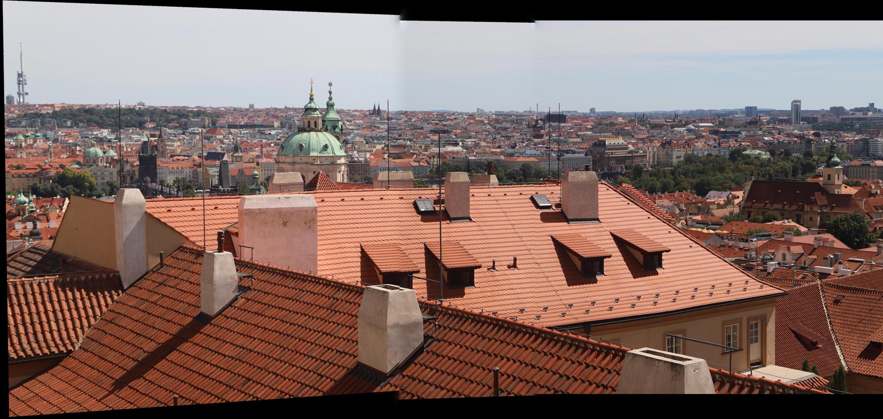
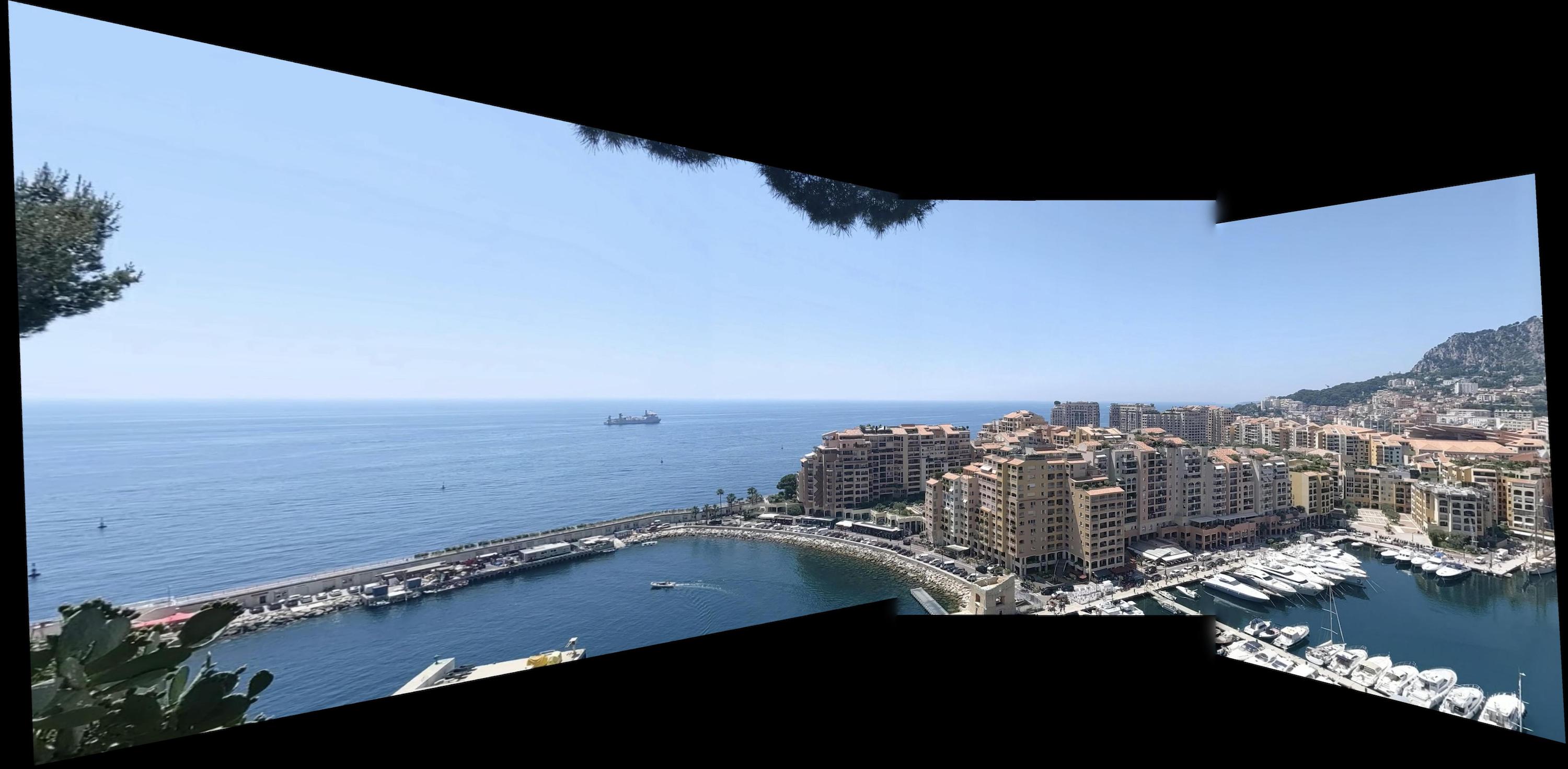
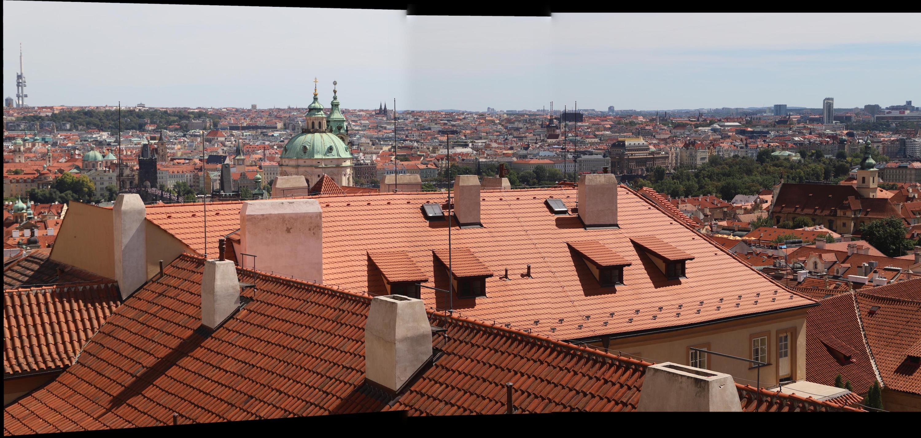
Now that we have figured out how to warp images, given three images from the same point of view, we can utilize our homography to create a mosaic of images. We will generate a black canvas and warp each image to a given reference image. In order to blend the images appropriately, we will use multiresolution blending.

City Photo Courtesy of Shivam Parikh:

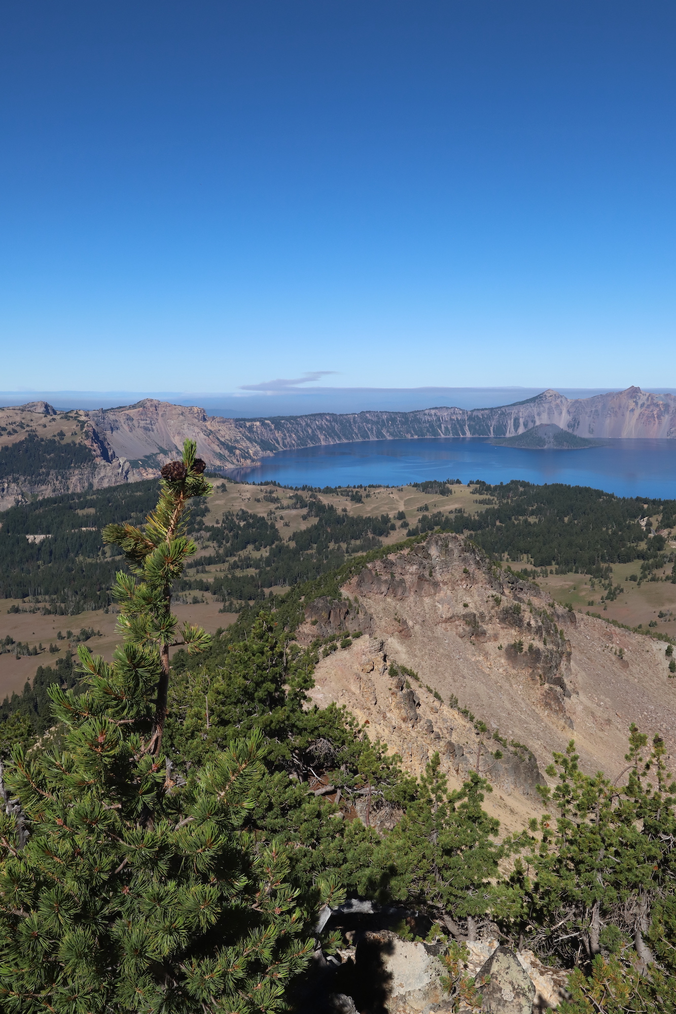
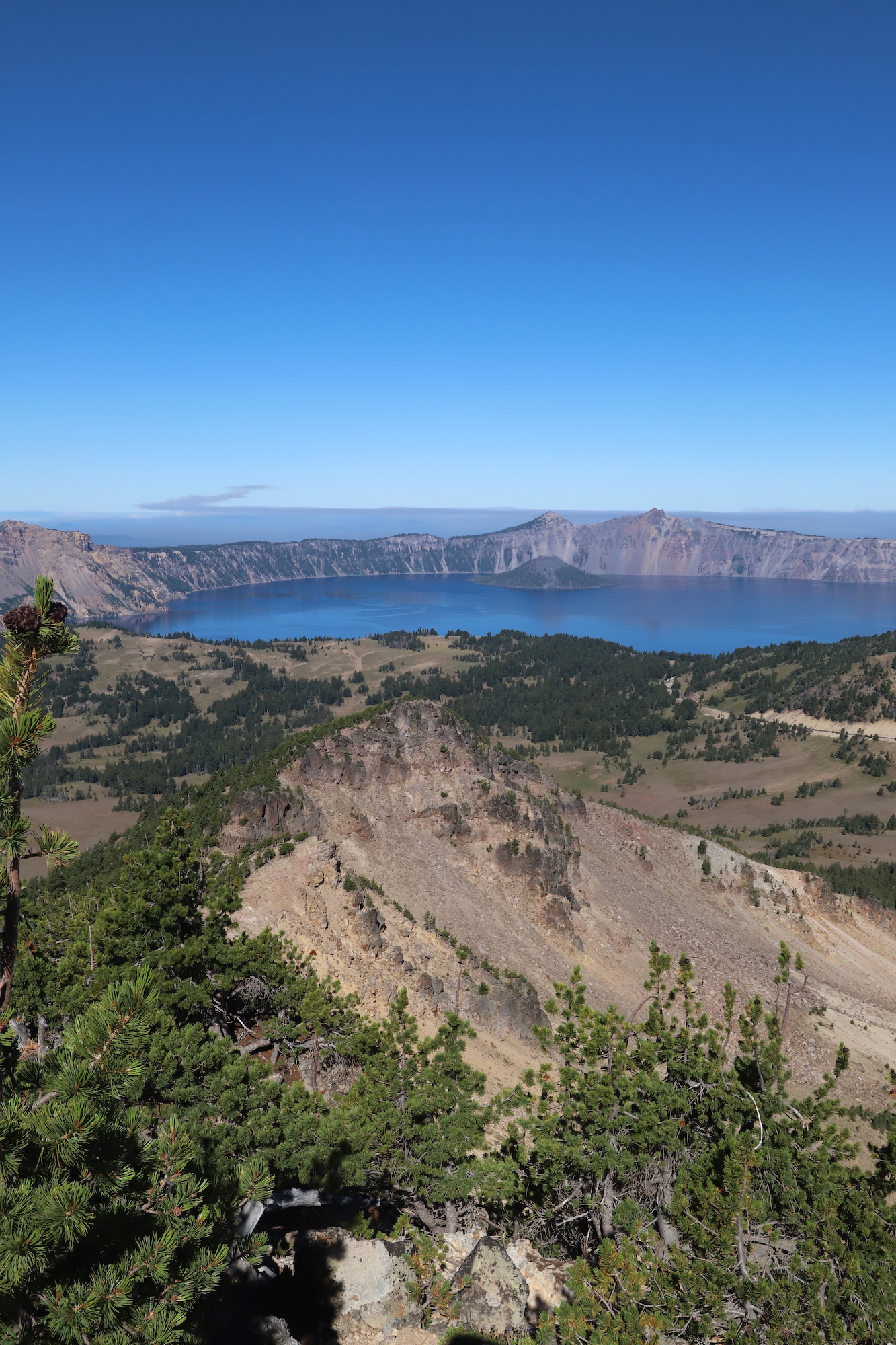
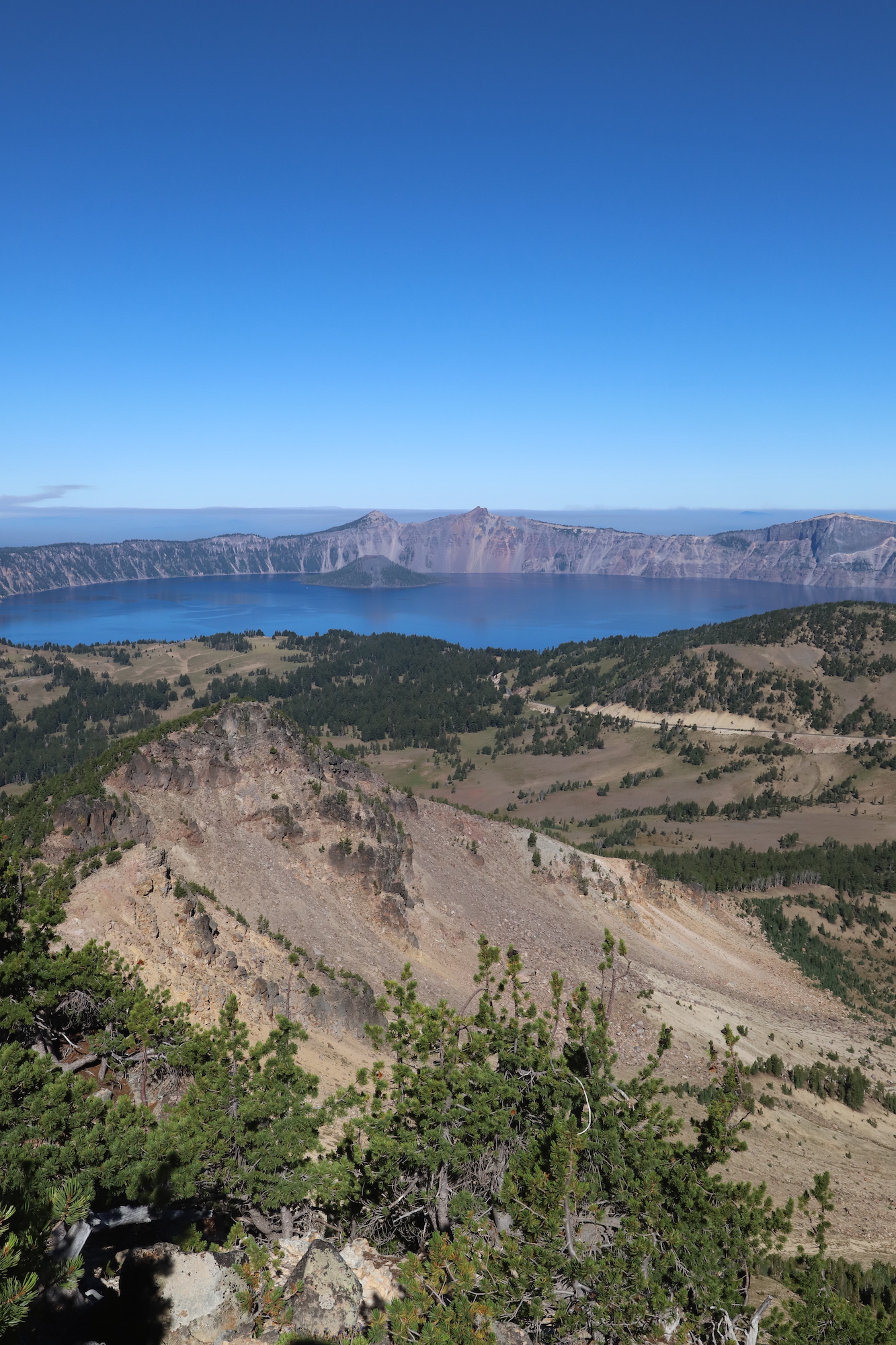
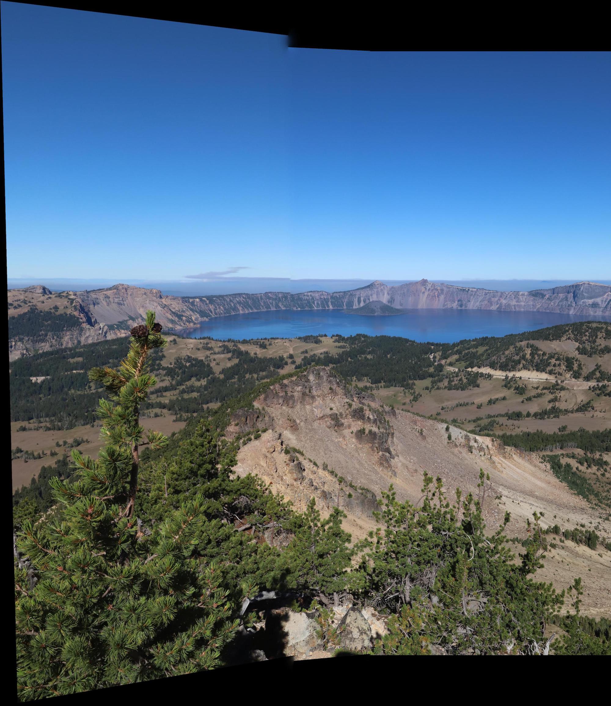
Lake Photo Courtesy of Shivam Parikh:

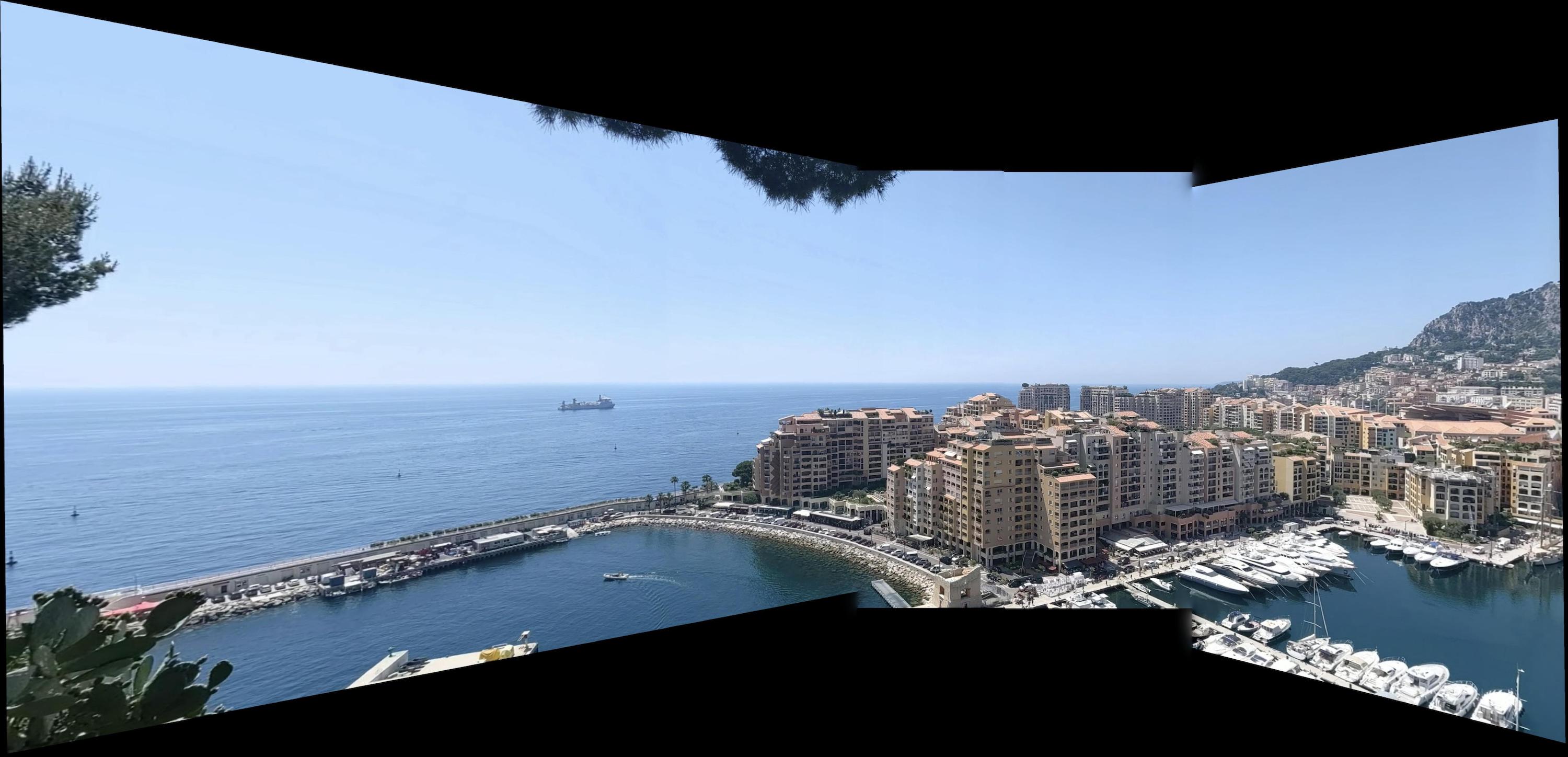
Monte Carlo Courtesy of Myself:

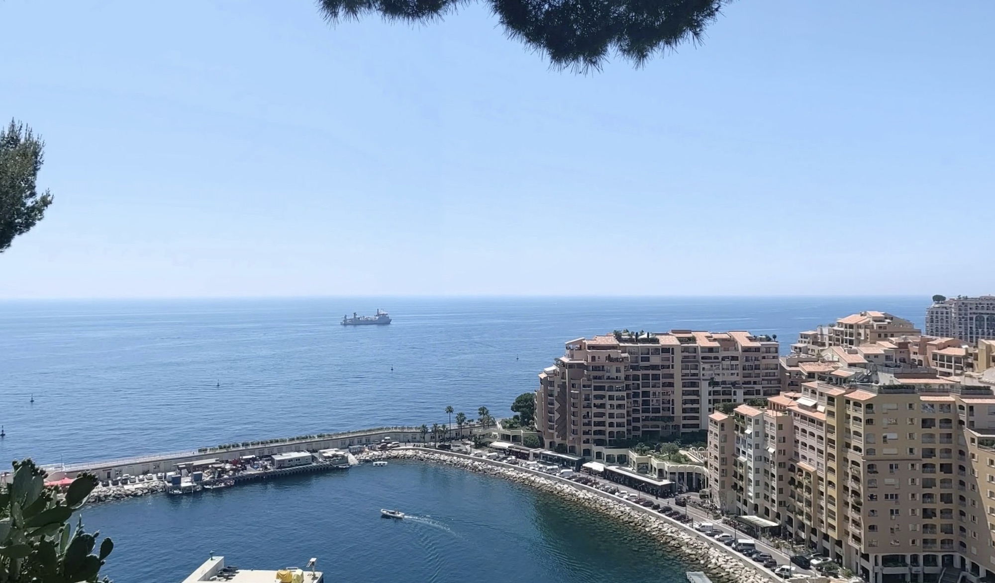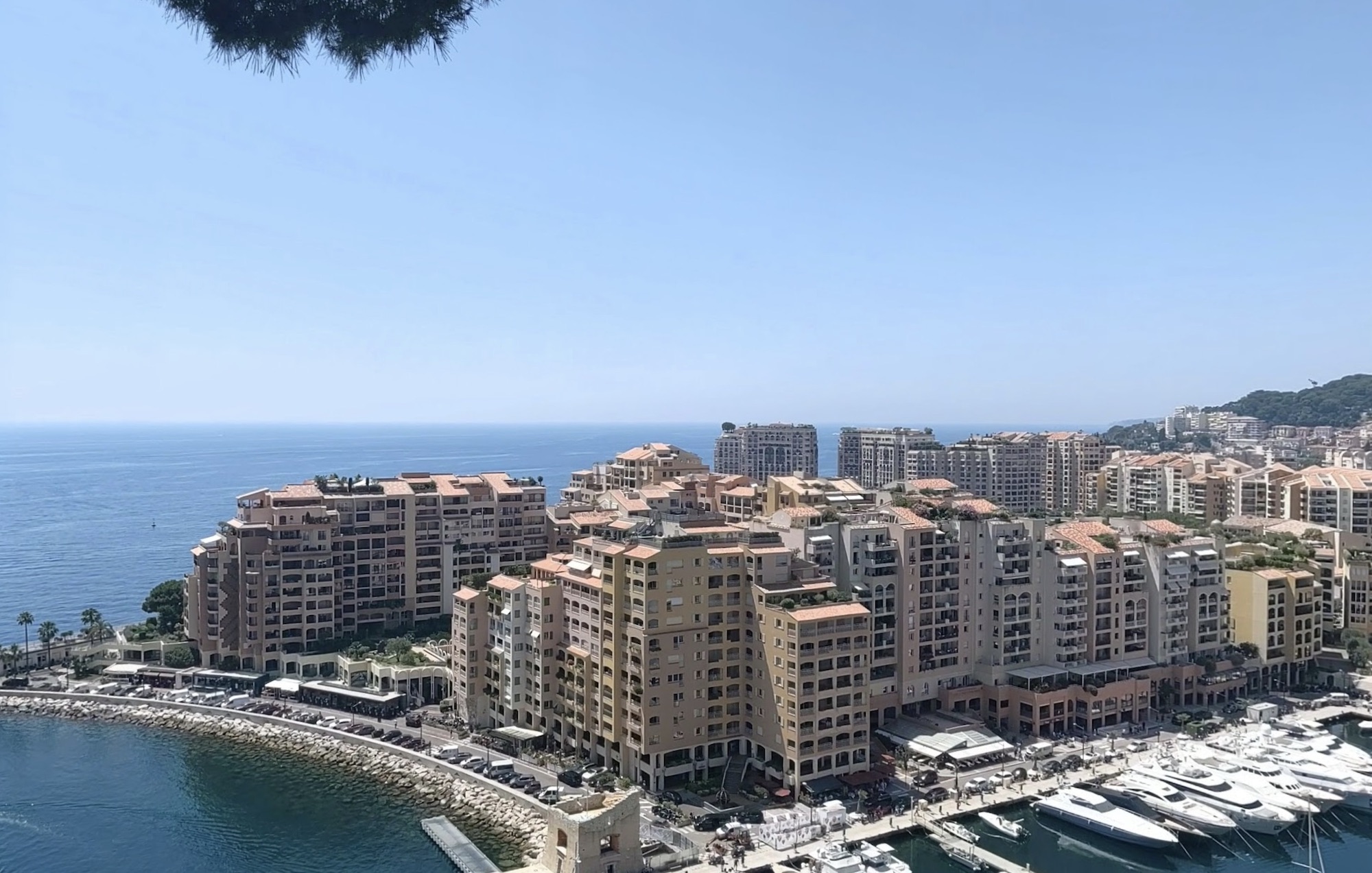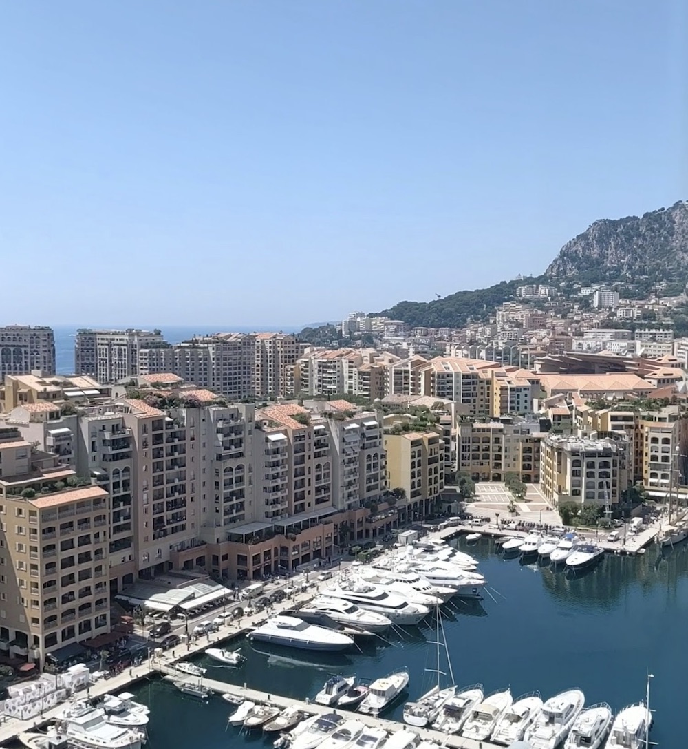Part 2: Automatic Stitching

We will be using a simplified implementation of this paper to automate correspondence determination.

Harris Corners

We will be using Harris corners to find matches between images. Corners are suitable to this end, because they are uniquely identifiable. Edges, on the other hand, do not have a unique point location that can be cross-referenced between images.

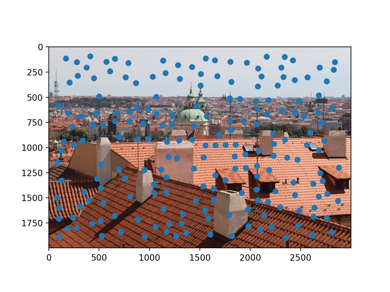
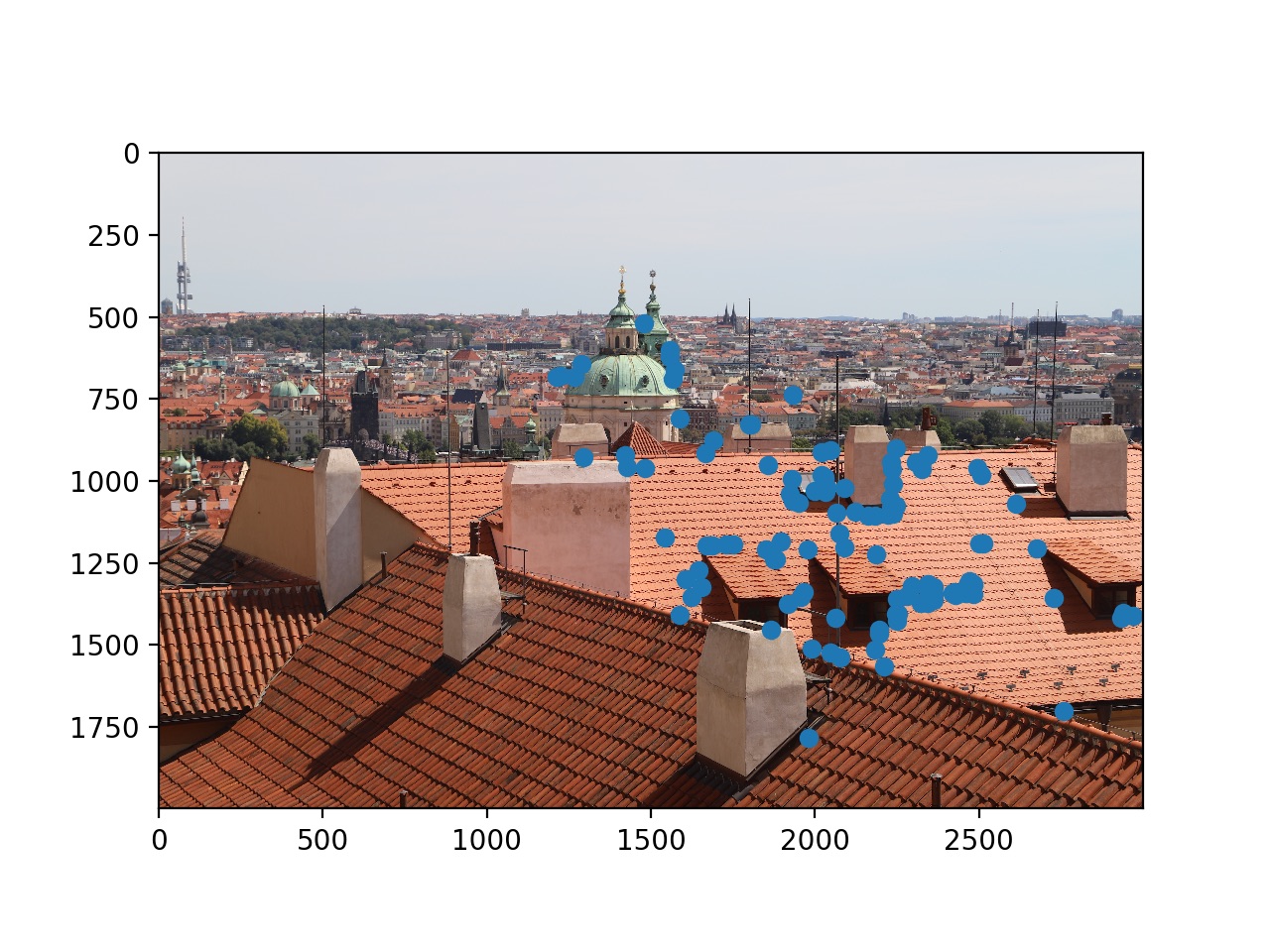
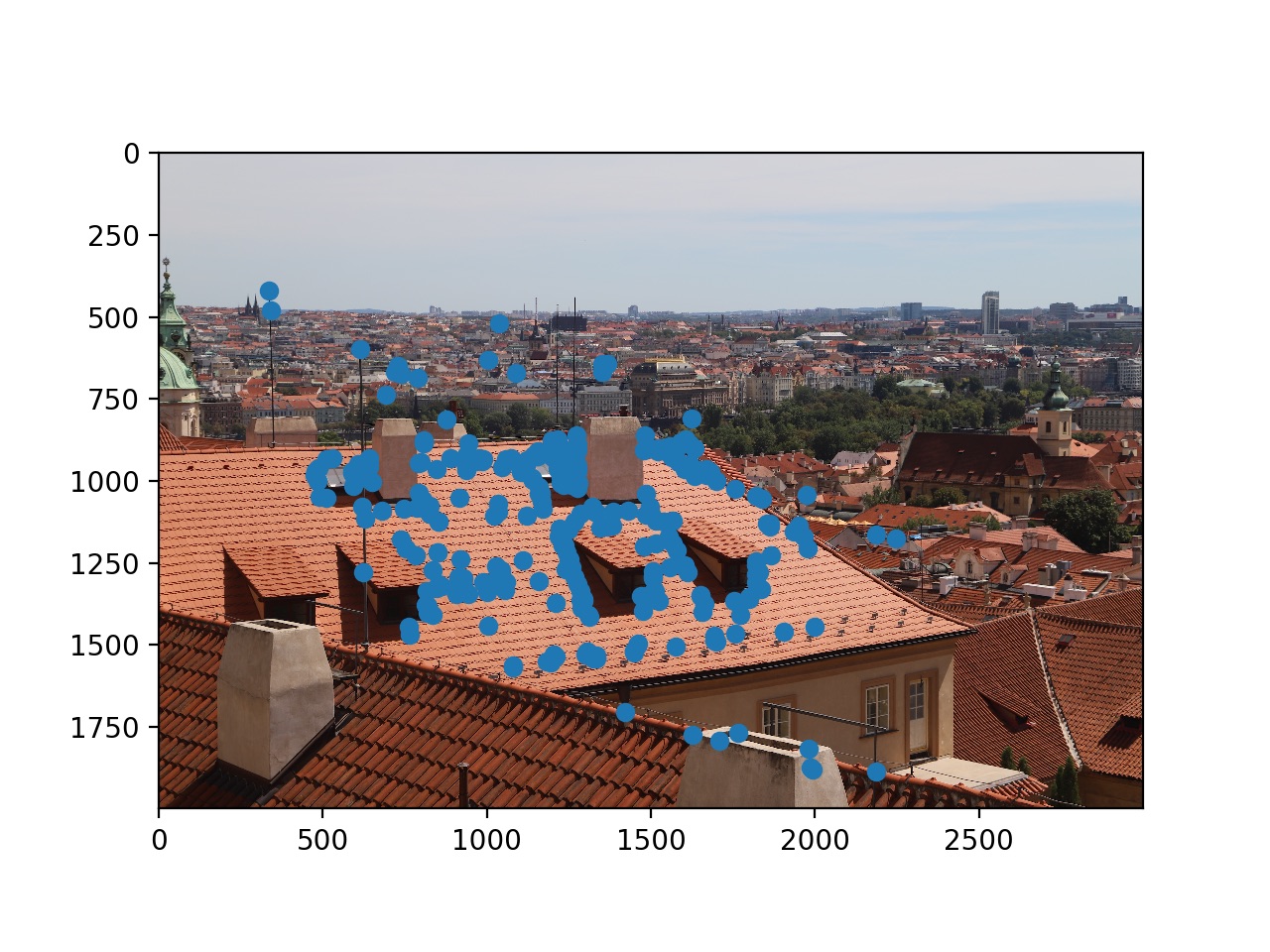
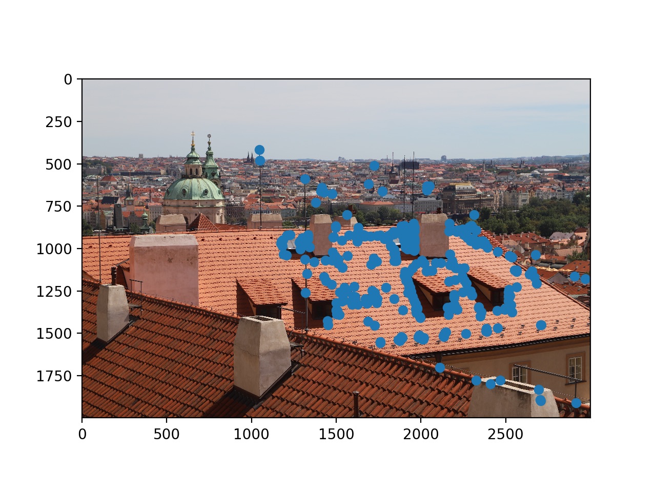
Shown below are the Harris Corners for an image of a city (courtesy of Shivam Parikh):

Limiting corners to one in every 75 pixels:

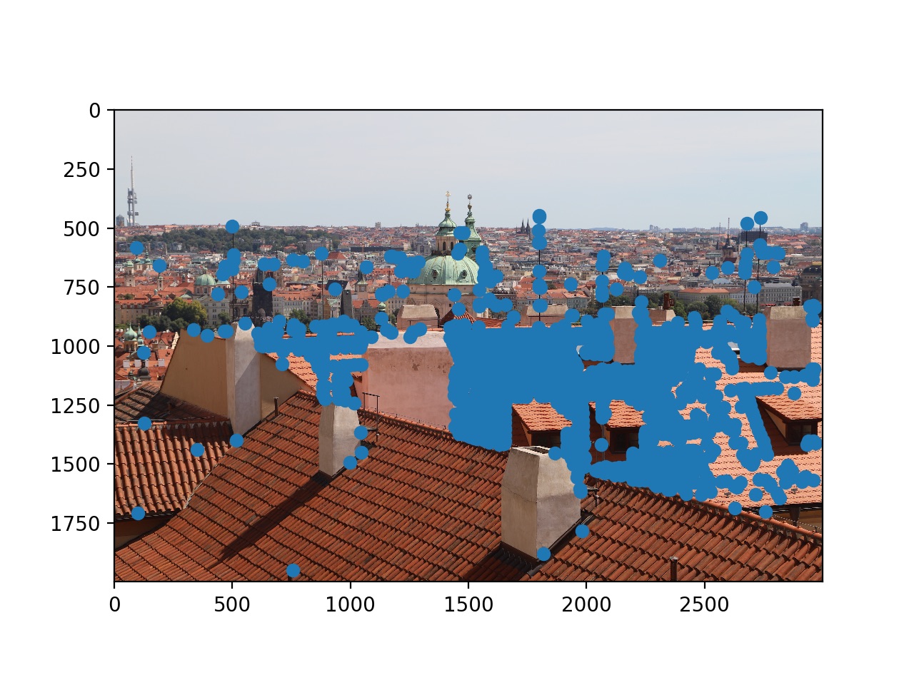
Adaptive Non-Maximal Suppression

Finding correspondence points is $O(N^2)$. Thus, it makes sense to reduce the amount of potential points that we will analyze. We will be using ANMS as described in the paper above. Basically, we are selecting points that have the greatest minimum suppression radius (meaning that the point has a harris value greater than $ c_{\text{robust}} \times$ that of all other surrounding points in that radius except for one point at that radius boundary.)
$[ r_i = \min_{j} | x_i - x_j |, \text{s.t. }f(x_i) < c_{\text{robust}} f(x_j), x_j \in \mathcal{I}$
We will be using a $c_{\text{robust}}$ value of 0.9 and keeping the top 1000 or so points.

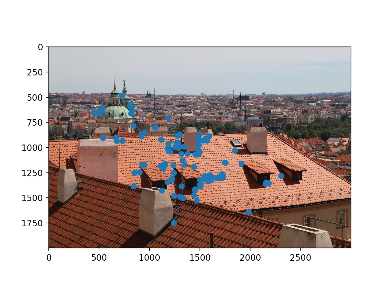
Chosen Points:

Feature Descriptors

We will now use the recovered points to define feature descriptors. We will use the surrounding 40x40 pixels centered around the point and downsample to an 8x8 (reducing noise/variations). We also subtract the mean and divide by the standard deviation to normalize and de-bias our feature descriptors.

Feature Matching

We will now use feature matching to find matches between the two images. We will vectorize the feature descriptors and subsequently find the SSD from every feature in the image to every feature in the second image. In accordance with the paper’s findings, we will use base our threshold for feature matching on the basis of the first and second best matches. ($\frac{1-NN}{2-NN} \leq 0.6$)
This idea is based on the Russian Grandmother Principle:

A true perfect match should only have one good match not multiple.

RANSAC

Finally, we will use RANSAC to ensure that we filter out any outliers in our data. One way to do this would be to manually run through all possible homographies and see which one results in the most matching correspondence points (within a certain threshold), but assuming that enough of our correspondence points are accurate to begin with, we can just randomize this process and with a large enough number of iterations, ensure that our final homography is accurate and filters out any outliers. Roughly 1000 iterations were used here. (I made it linearly increase according to correspondences.)

Final Results

Manual	Auto

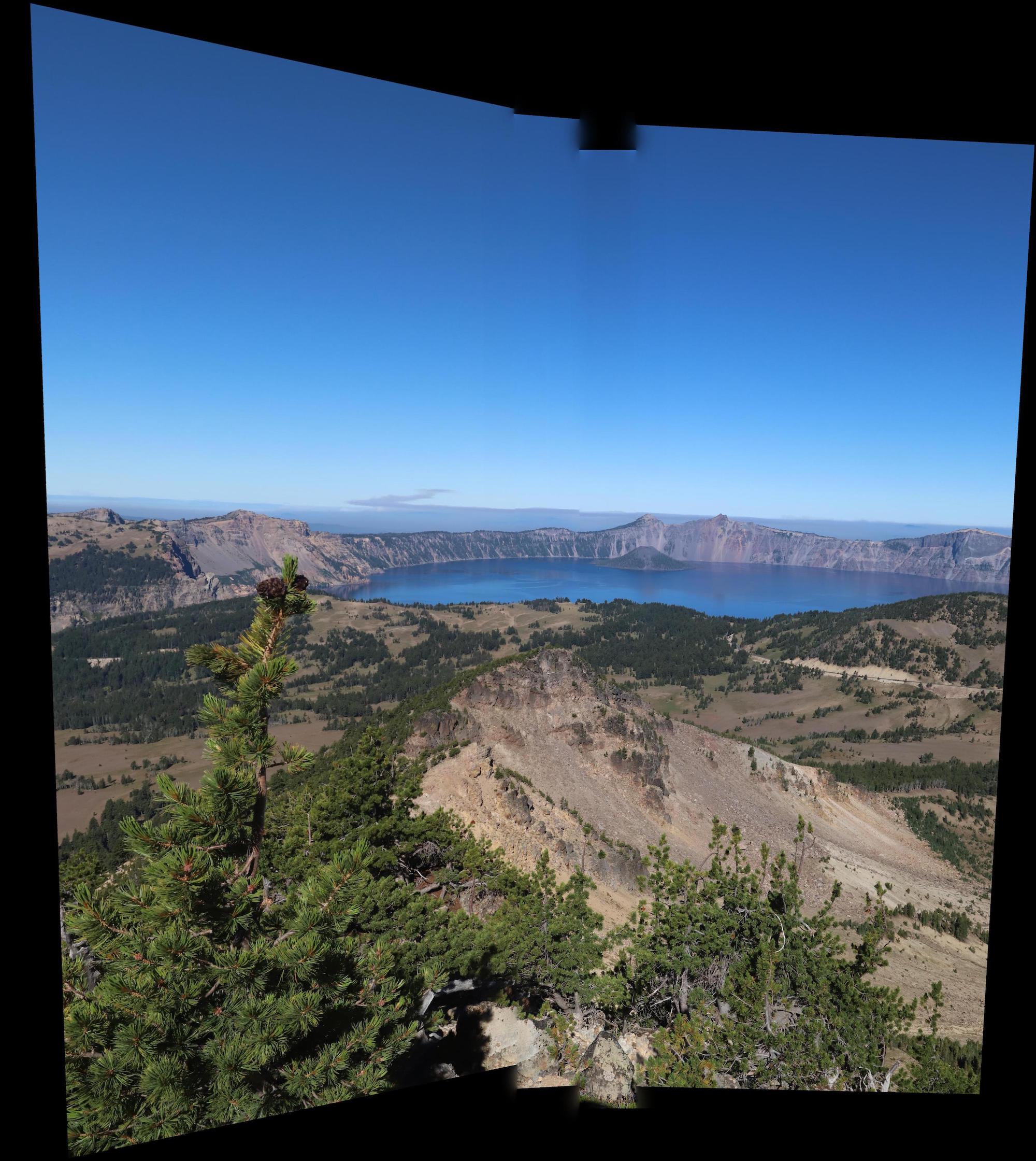
Huge Panorama for Lake:

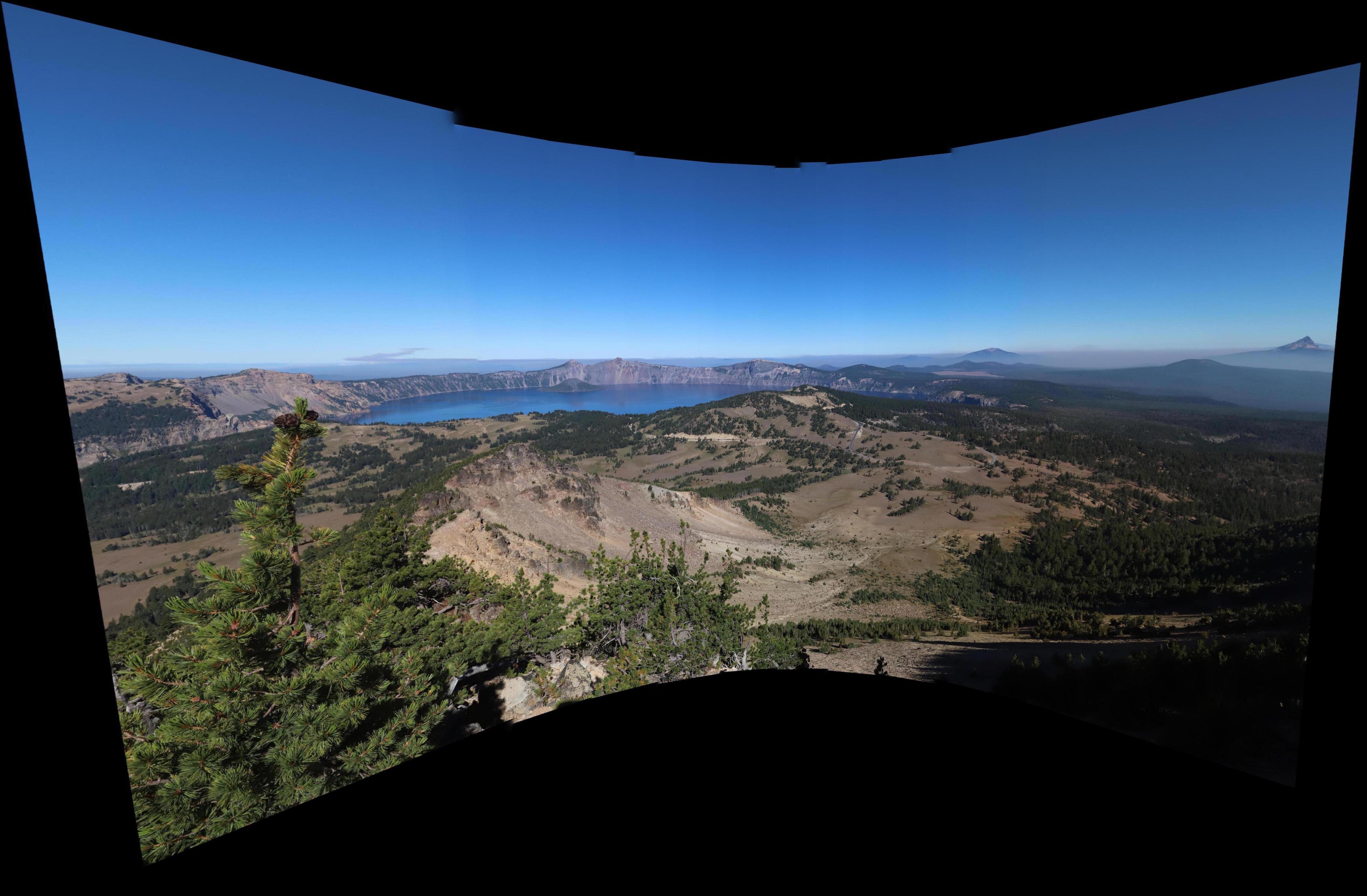
The results are mainly quite comparable. For the automatic lake, I did a projection of 0 onto 1 onto 2. However, I did a projection of 0 onto 1 and 2 onto 1 for manual. This resulted in slightly different results here. Otherwise, the correspondences turned out to work almost as good in manual if not sometimes worse.

Bells and Whistles

Rotation-Invariance

Using the derivative of the gradient, I calculated the general direction of each feature descriptor and subsequently rotated them as to ensure that any two feature maps would have the same alignment. My feature descriptors are also fully RGB.

Original	Invariant

Polar Warping

I did a polar warp of Obama as to generate anamorphic art, similar to that of Istvan Orosz. (More on that below.)

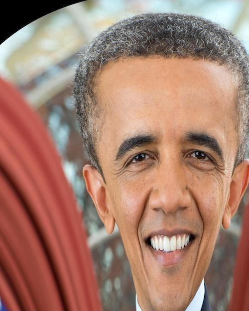
Cycle-GAN with Polar Warp

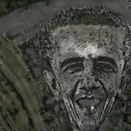
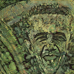
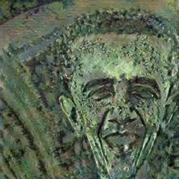
I did a polar warp of Obama (cut off the black parts of the polar warp). I then fed the resulting image into Cycle-GAN (map2sat). Although the photograph was not a map, the GAN was able to hallucinate a map on Obama’s face and subsequently turn him into a satellite image. I then subsequently fed this satellite image into other Cycle-GAN (style-monet and style-vangogh) to create two artistically styled, anamorphic posters of Obama. Given more time, I think I could mess around with GANs and produce some more interesting results.
Satellite:

Van Gogh:

Monet:

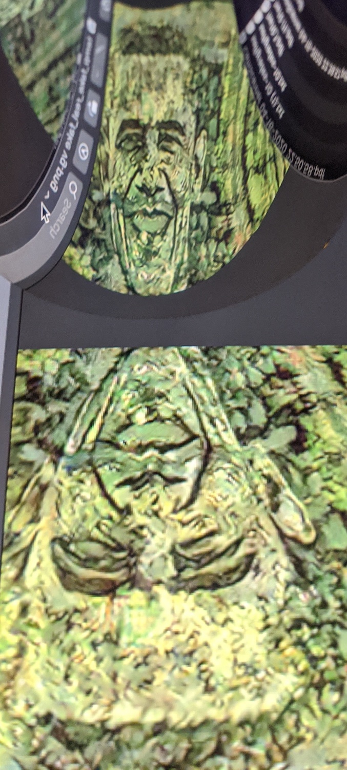
Anamorphic (Using a reflective cylinder):

What I learned

I learned feature extraction, warping with homographies, and various feature matching tools. I’ve always wanted to learn how to make CamScanner 2.0, and I guess I’ve finally achieved that.