Part 1
The purpose of this part of the project is to understand homographies and transform images into mosaics. This employs a different method of image transformation we have not worked with before.
Recovering Homographies
A homography is a type of transformation with 8 degrees of freedom. We will be applying this transformation to our photos such that they may be manipulated for image rectification and, later, mosaics. Our first step in this process is finding the parameters of H, the homography matrix for the transformation. Below is a snapshot of the matrix equation of homography. This is taken from
this lecture from a course at Penn State.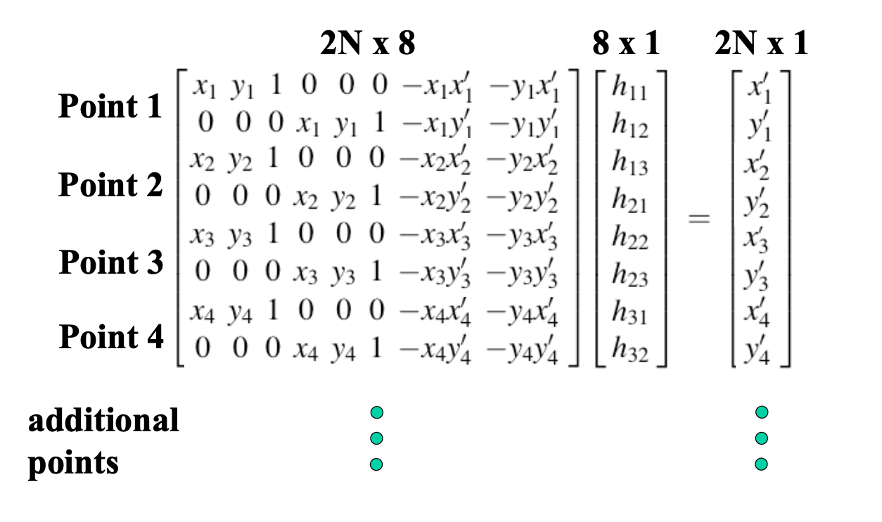
The input to our function computeH takes in two parameters: correspondence points from a "before" image and correspondence points from an "after" image. We use these points in a system of equations to solve for the 8 parameters of the H matrix. Using the equation setup from above, we solve our system using least squares. This solution provides us with the inputs for the transformation matrix H.
Image Warping
After receiving our transformation matrix, we work on transforming the images in order to rectify them. I had a lot of trouble with this portion of the assignment because I felt that x and y values needed to be swapped and played around with to get successful results. My process for this part was to receive all of the pixels within an image and apply the transformation H to them via dot product. It was necessary to "normalize" the values received from the output of this dot product because each pixel coordinate was scaled by some w, which was also found by the dot product. After dividing both the x and y coordinate by this w value, we were able to receive the translated coordinate, thus successfully transforming the image to new shape to accommodate the rectangle.
Image Rectification
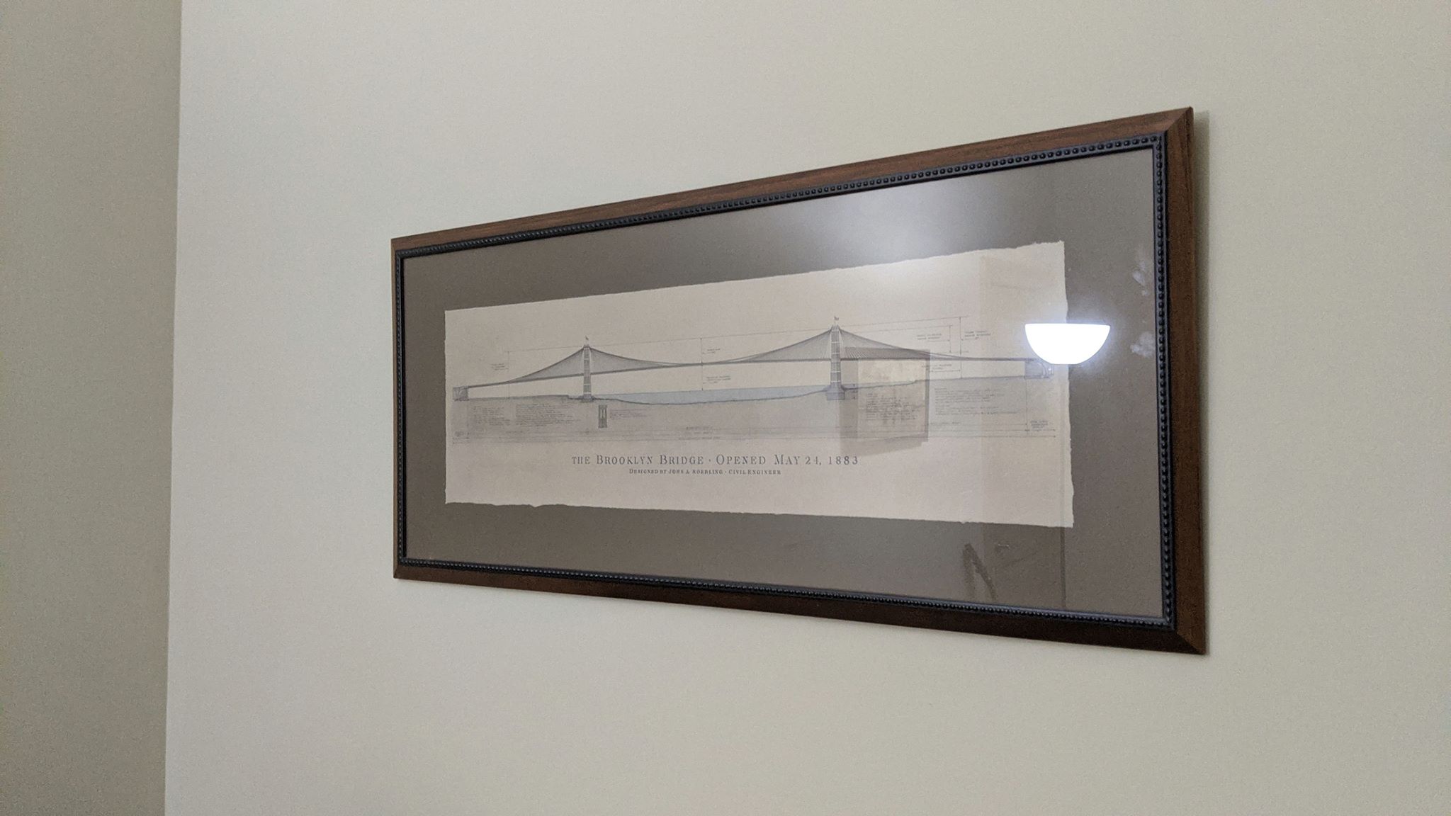
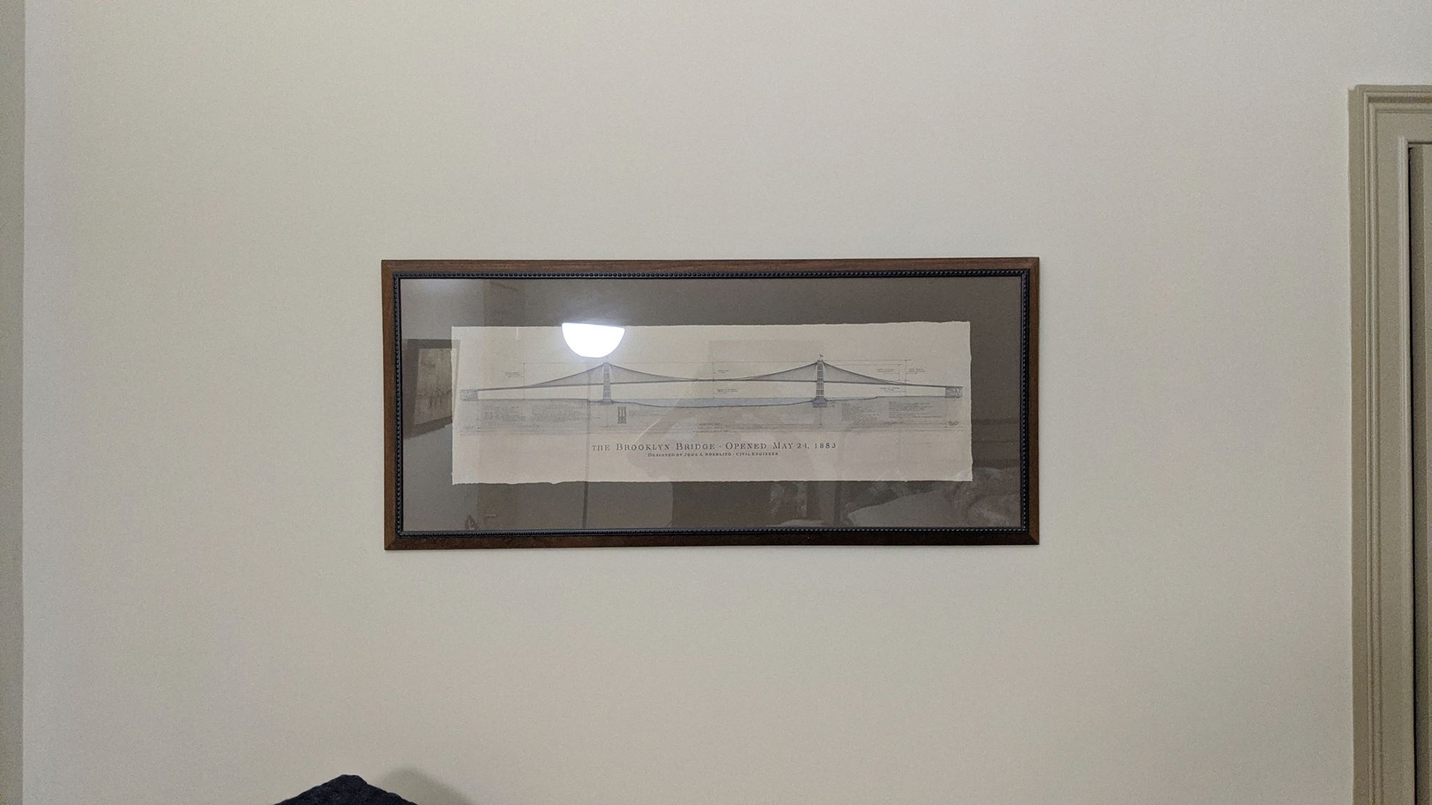
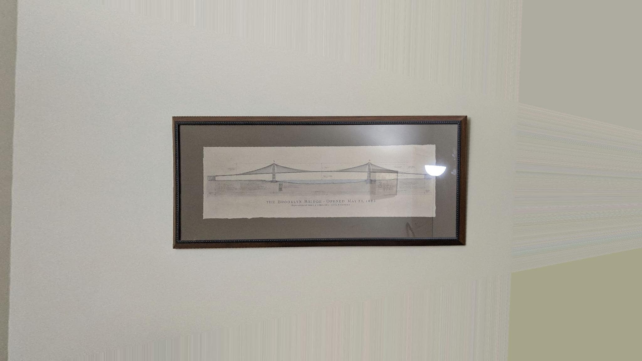
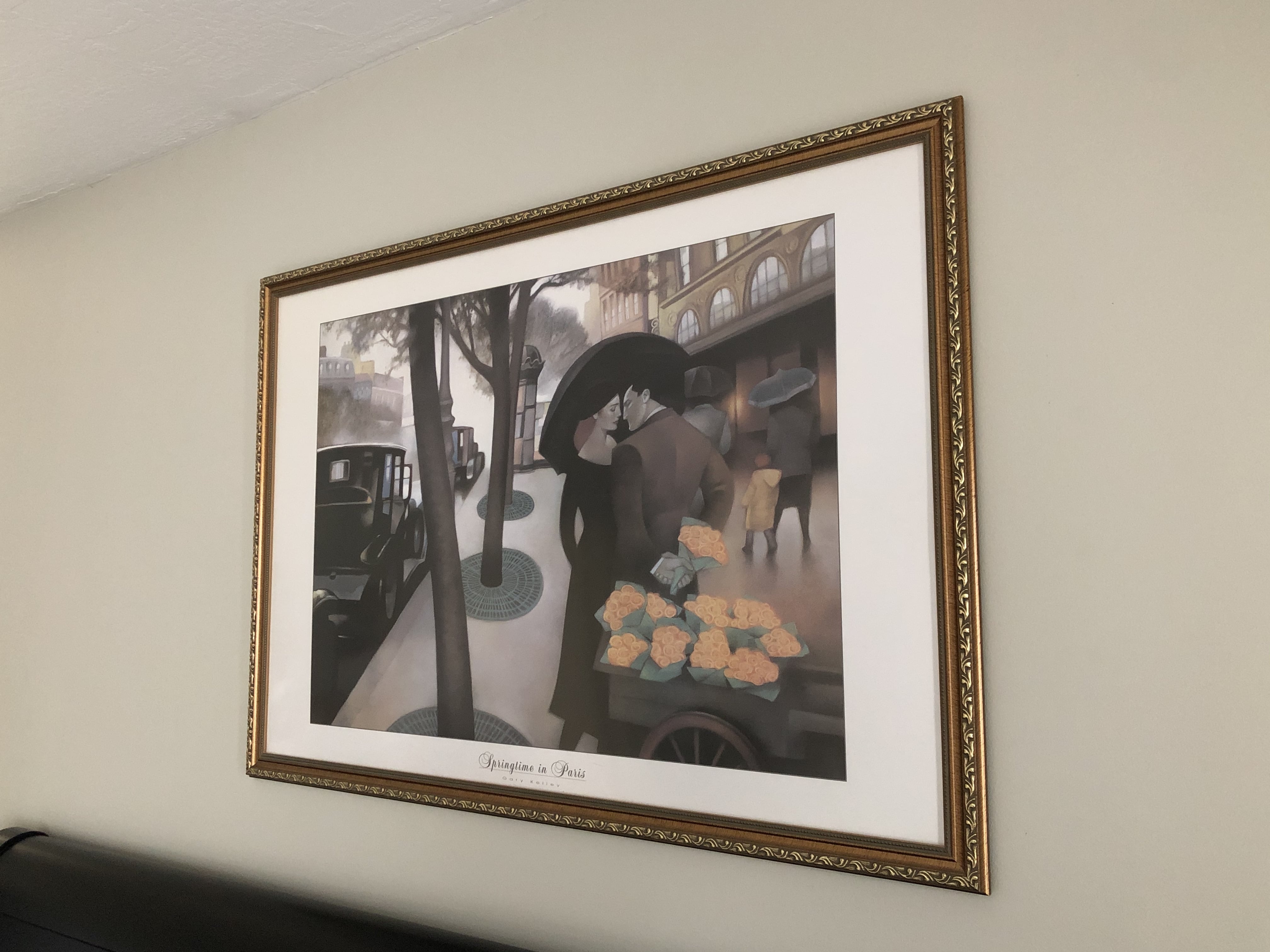
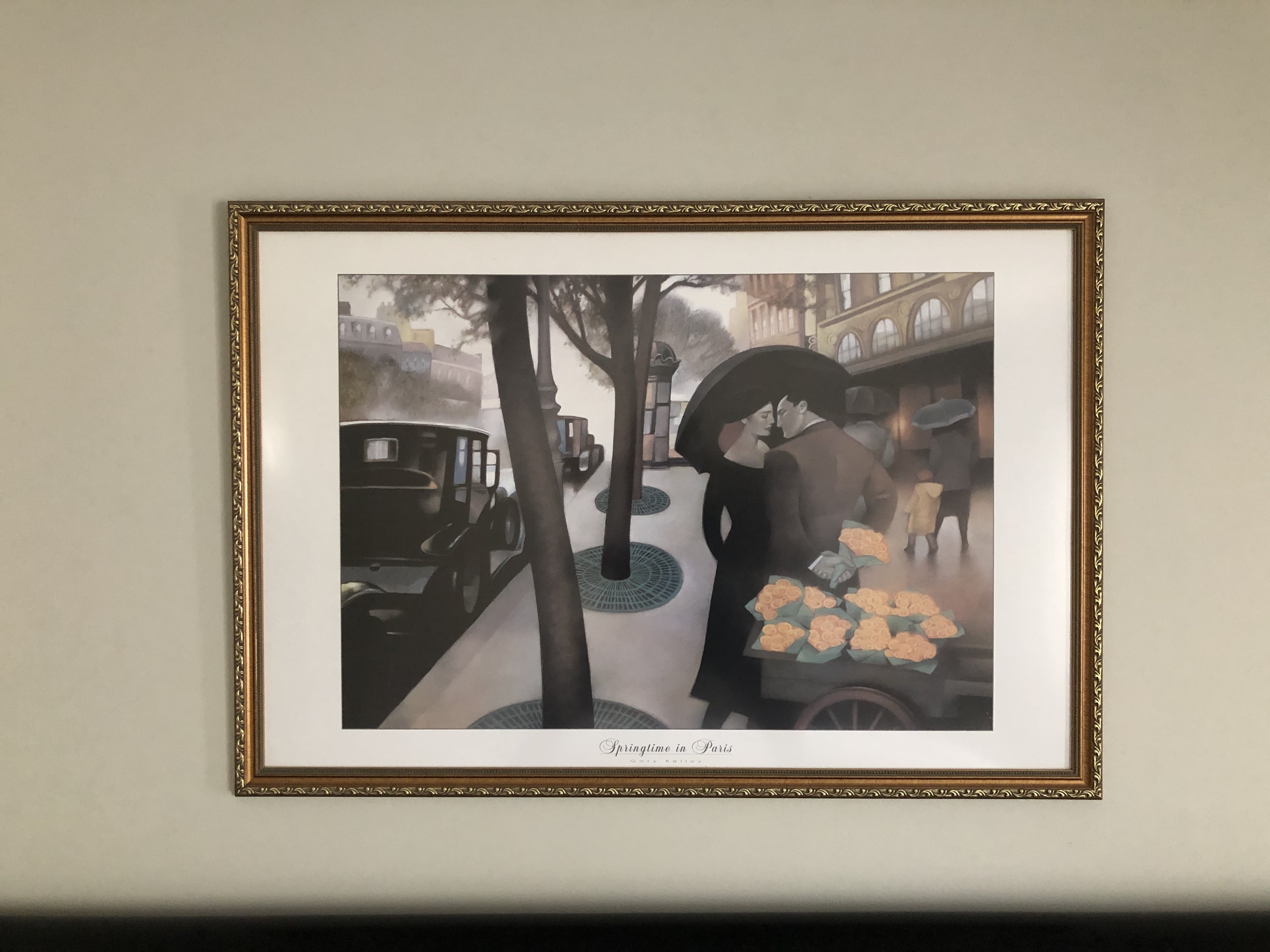
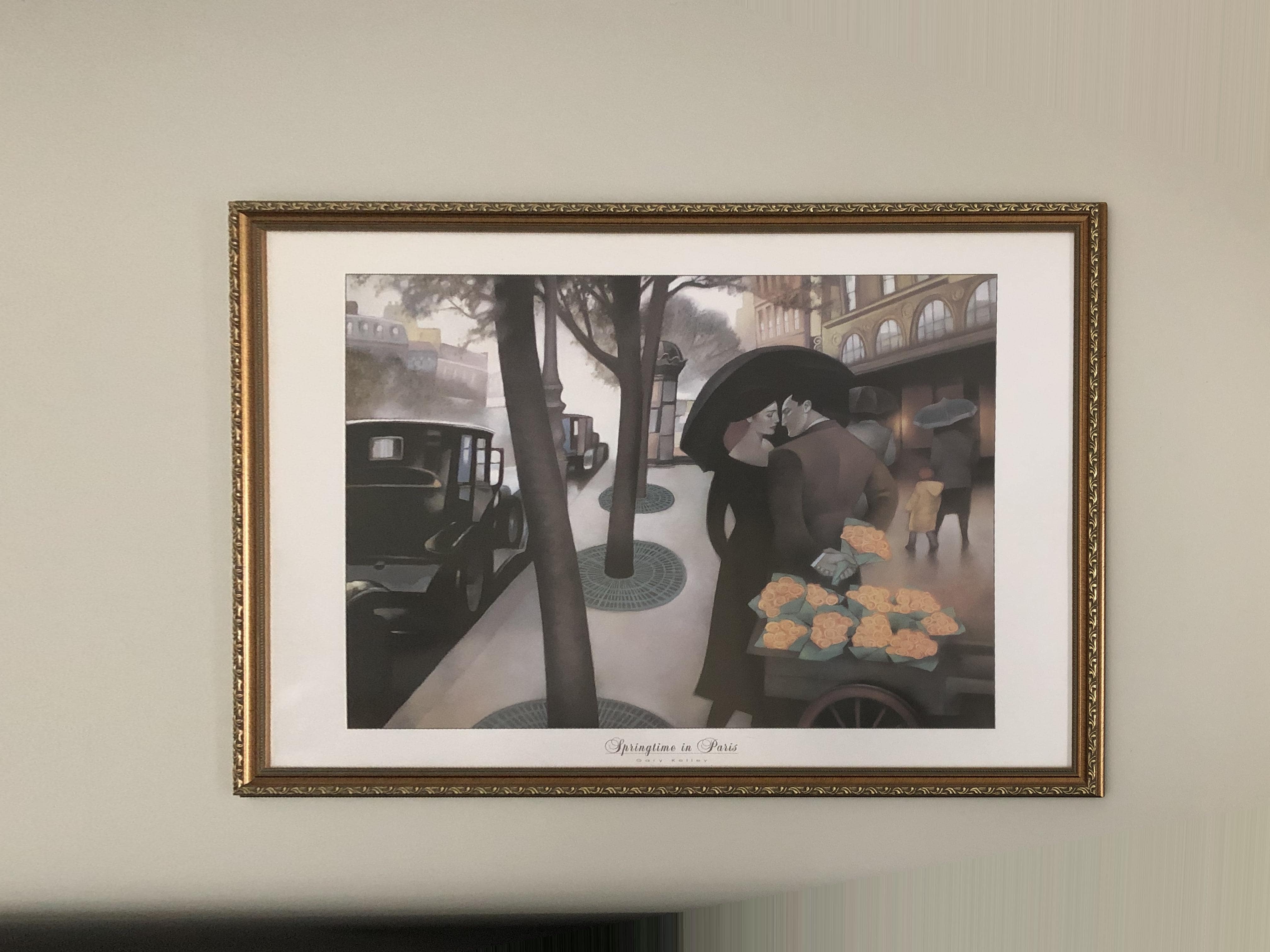
Below are some results of my image rectification. I was quite pleased with the results using standard rectangles, or in this case, paintings.
Bridge
Springtime
Curved Monitor
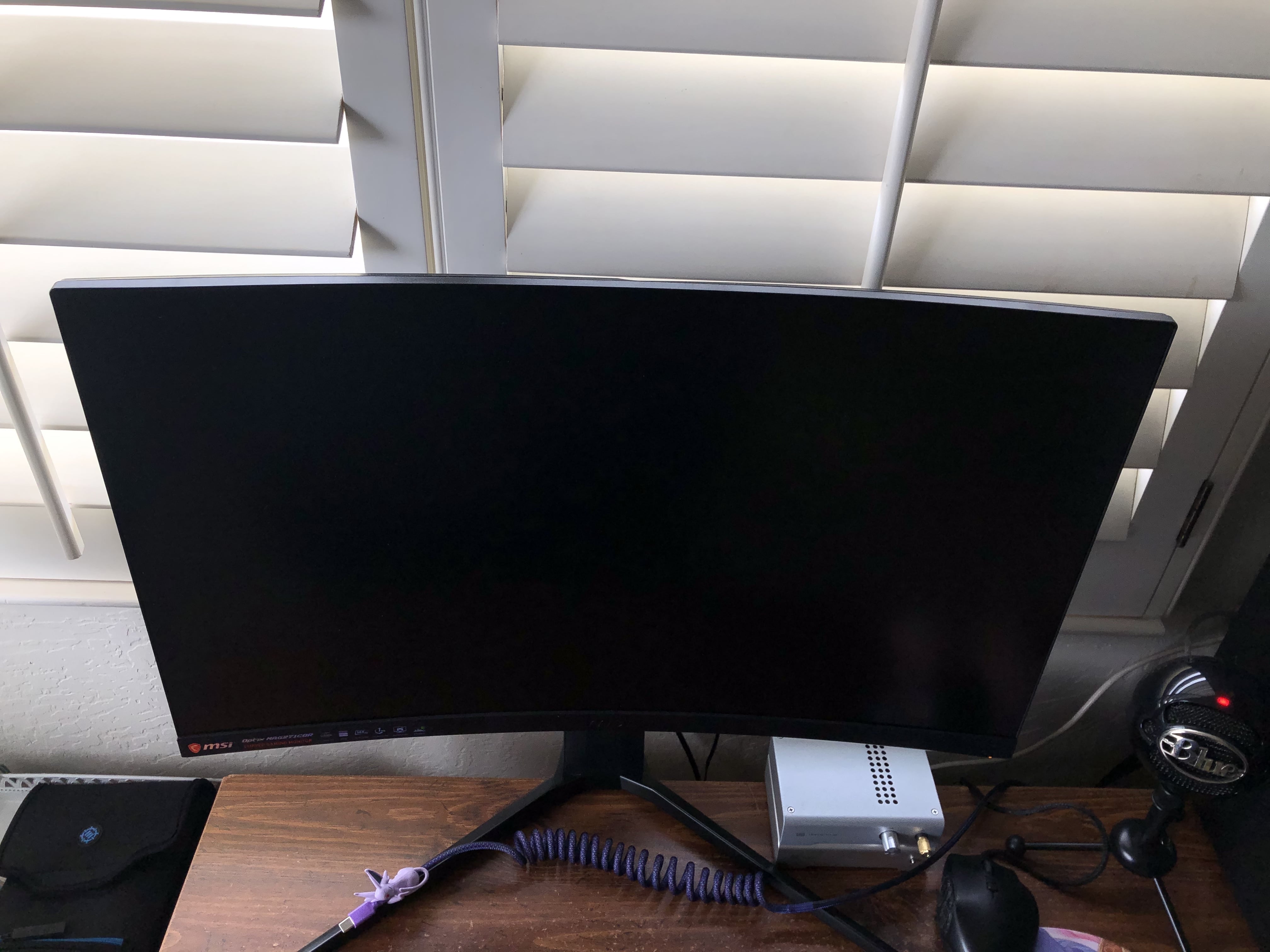
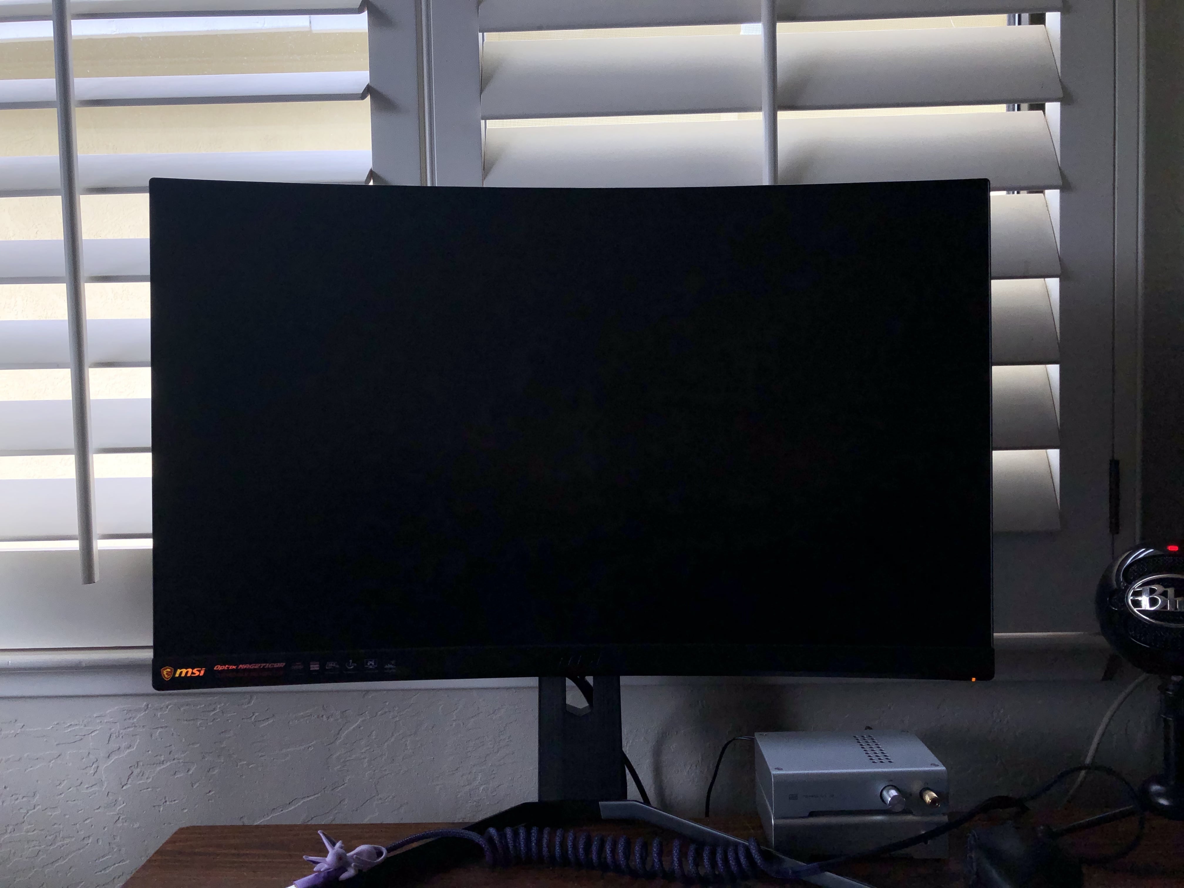
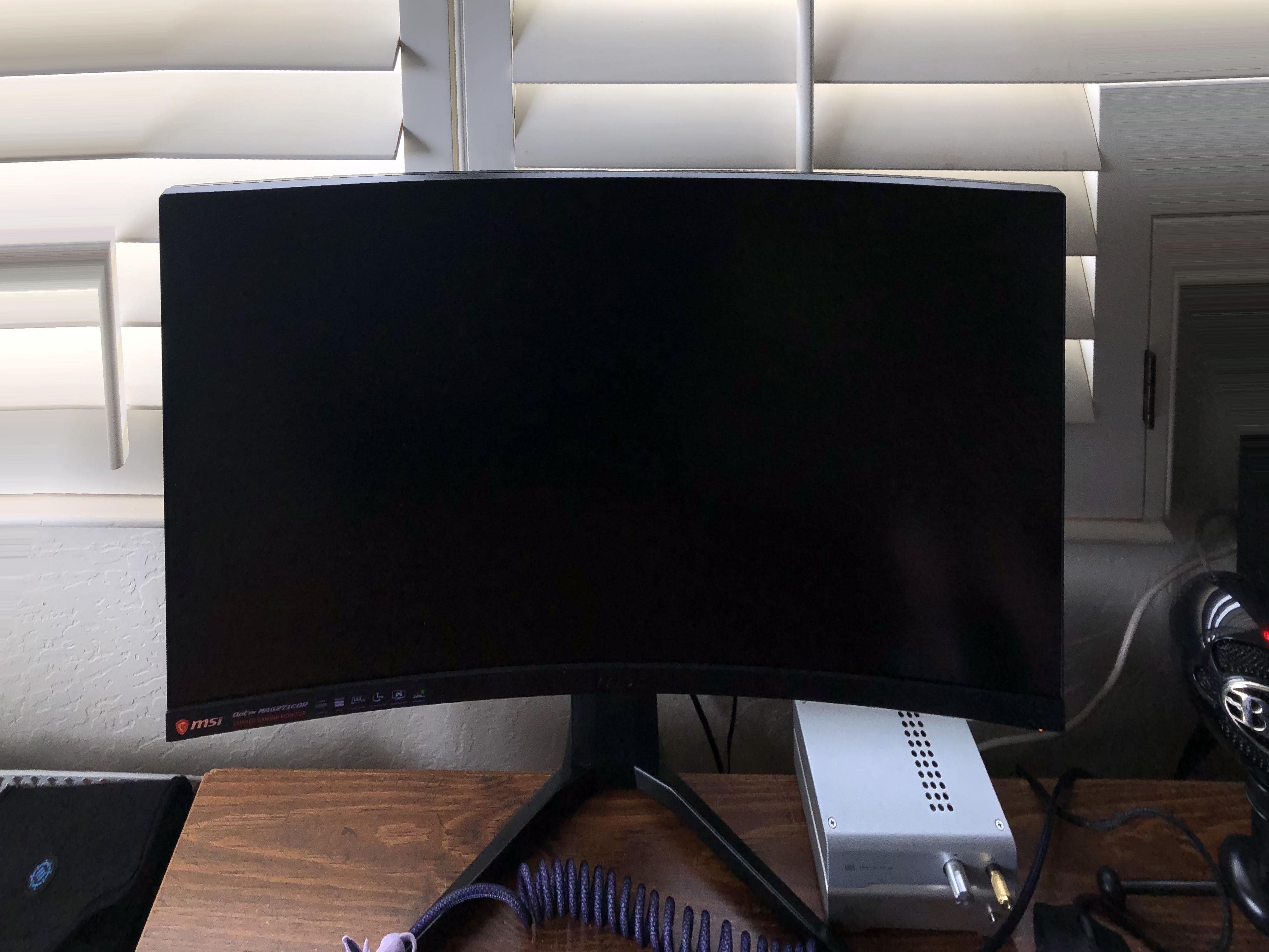
I included this set of images because I thought it was funny how the rectification came out. Since the monitor is not a perfect rectangle, the resulting warping image came out a bit funnier than the rest. It looks like you have to choose objects in photos with good rectangular shape to produce well-blended images.
Photo Mosaics
After working more on image warping and output shape, I was able to produce manual photo mosaics with some images. Again, huge credit to fellow student Kenny Chen for assisting me with this part of the project and talking out issues with me. Even after Part 2, image mosaics gave me the most trouble.
City
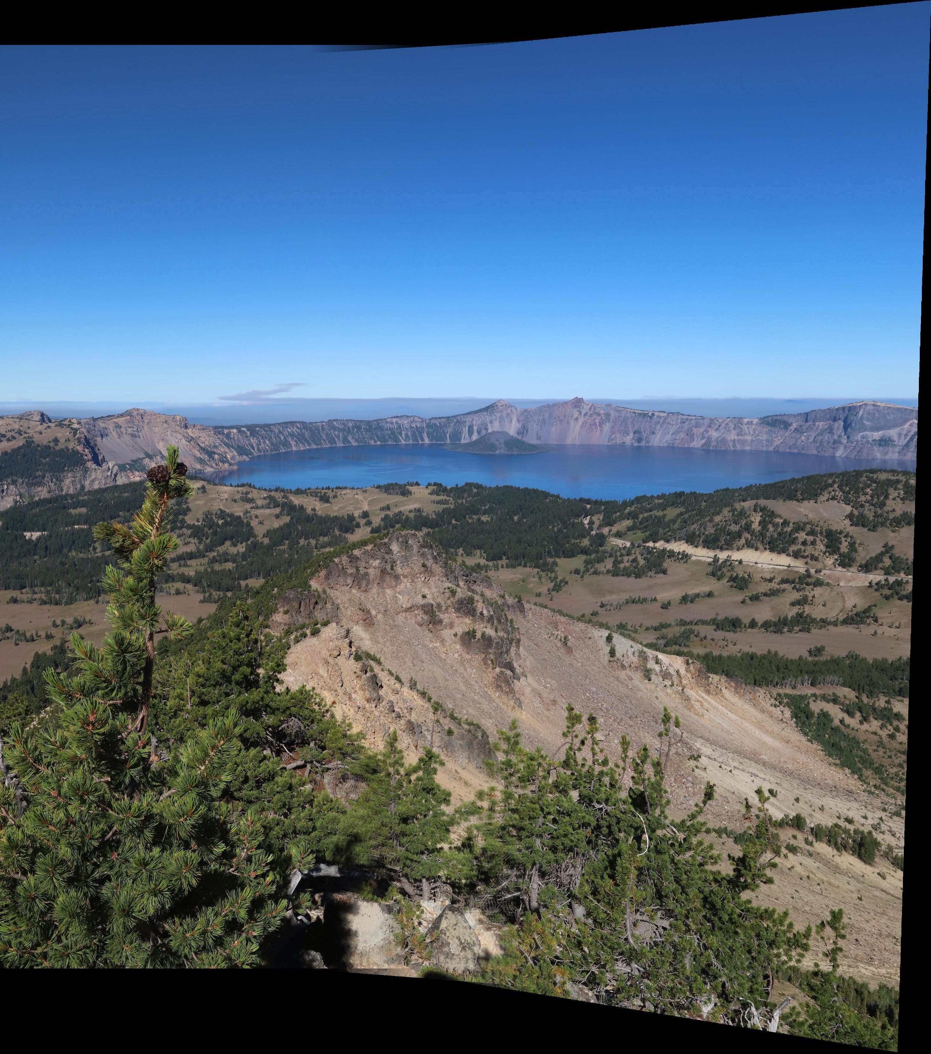
Lake
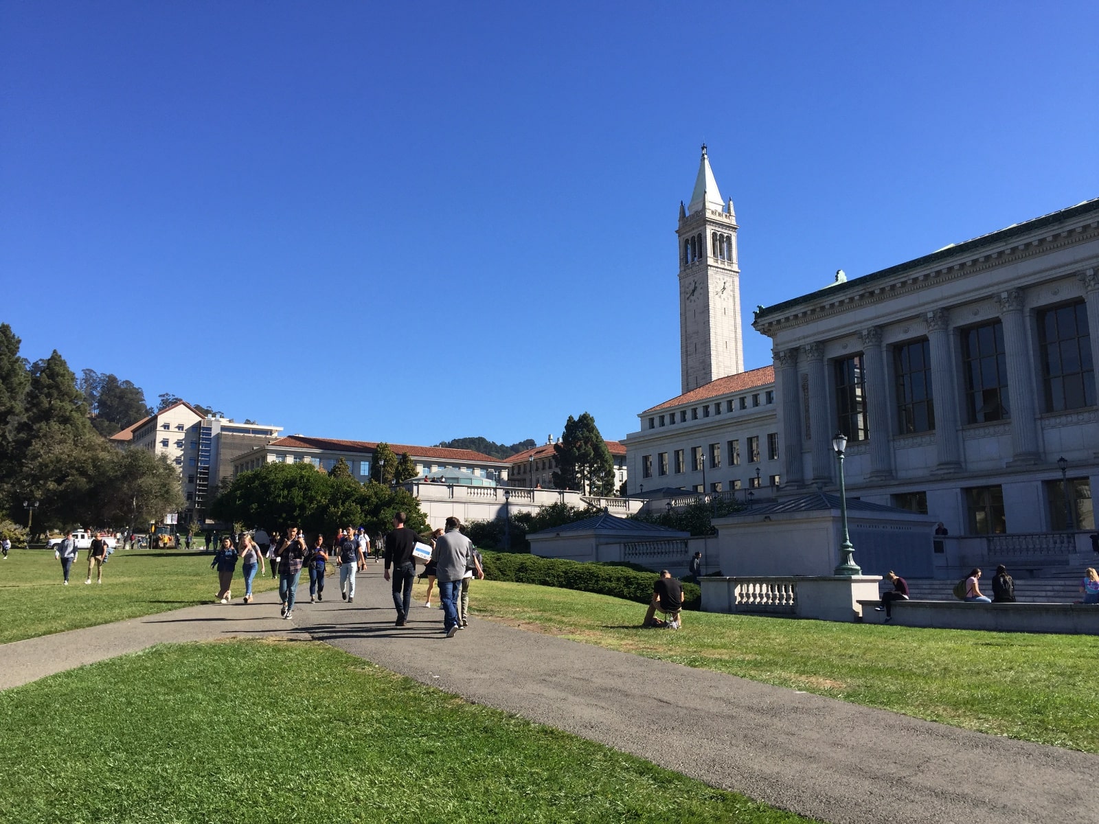
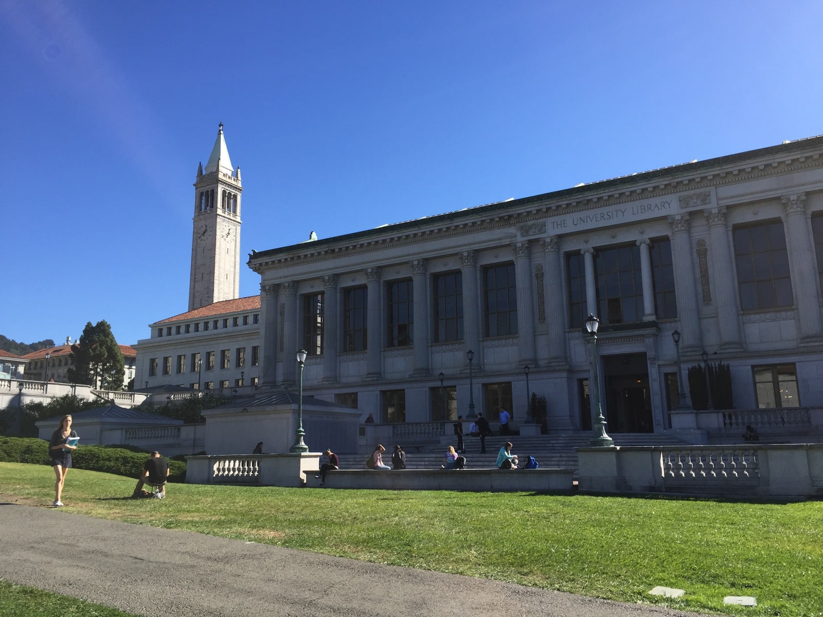
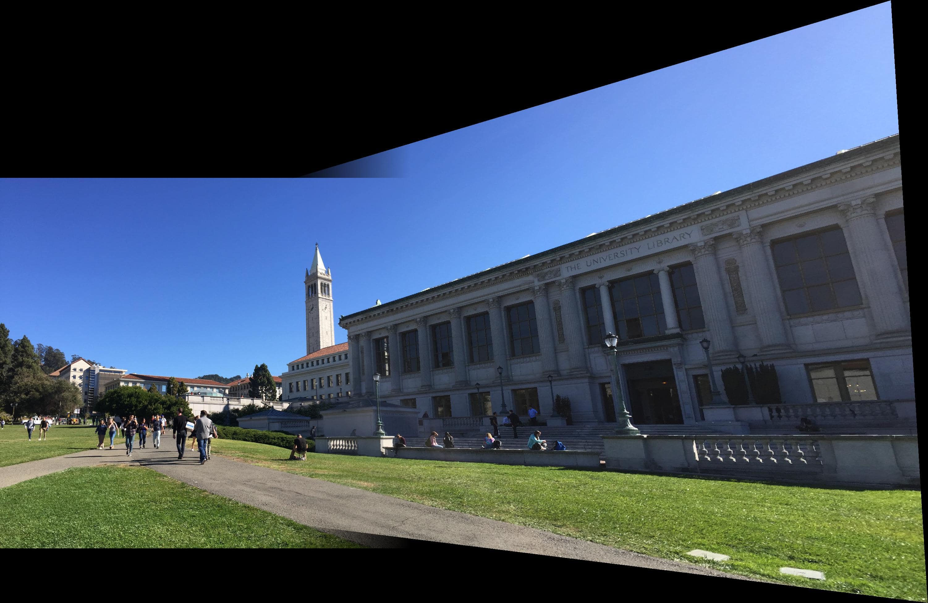
Memorial Glade
Images from Andrew Campbell (Fall 18).
Part 2
Harris Interest Point Selection
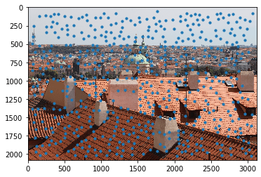
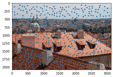
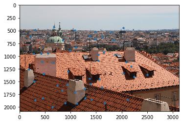
To start part 2 of the assignment, I used the starter code provided by the course staff. This code takes in a grayscale image and finds potential points of interest for feature matching. In order to reduce the number of points, I altered the min_distance parameter in the peak_local_max function. I set this minimum distance to 50 such that points will be somewhat separated. Below is the result of finding Harris corners on two input images (provided by Shivam).
Adaptive Non-Maximal Suppression (ANMS)
After getting a large number of points, I implemented Adaptive Non-Maximal Suppression in order to decrease the number of potential feature points, such that further code would have less points to go through. The process of ANMS is as follow:
- Loop through all points.
- Compare "cornerness" to all other surrounding points and take neighboring point with closest Euclidean distance.
- Sort points by distance in decreasing order (highest to lowest).
- Take n points with the furthest distances.


Feature Matching
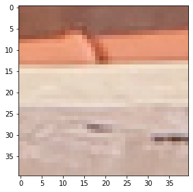
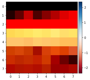
Even after the reduction of points, there is still room for error, where certain point pairings do not match up. In feature matching, we take a 40x40 feature box of pixels surrounding a point, resample it down to a 8x8 square, normalize it, and compare it to the feature boxes of all points in a second image. We do this to try to find the closest point matches between the two images. Below, we can see an example of 40x40 feature box and an 8x8 feature box that has been sampled down.
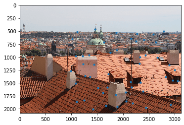
For each point, we record its relative error in comparison to all points in the second image. We are mostly interested in the lowest error and the second lowest error. If the (lowest error / second lowest error) is less than some threshold, we take the point pairing in question. If not, we do not accept these points into our final list of feature point pairings. Below are the results when performing Feature Matching. We can see that we have a lot of good points that look like they're in the same location in both images. This is a good starting point for RANSAC.
RANSAC
Even after reducing the number of feature points, there is still room for error with outliers in our points. In the images about, you see a selected point that sits in the sky, which would not be a very good point for when computing a homography. We now use RANSAC, a robust algorithm that selects points for computing an accurate homography and gets rid of outliers that may not be beneficial. The process for RANSAC is as follows:
- Select 4 feature point pairs at random.
- Compute a homography matrix using those 4 points.
- Apply this homography matrix to all feature pair points provided as input.
- Record the error (distance from paired point) for each point in the first image.
- Keep note of all points that produce an error under a specified threshold value.
- Continuously update a list of inliers, or points that produce an error under the threshold.
- If the number of inliers in the current iteration is larger than the previous, retain those points.
- Return the selected points that produced the longest list of inliers.


Auto-Stitched Mosaic Examples
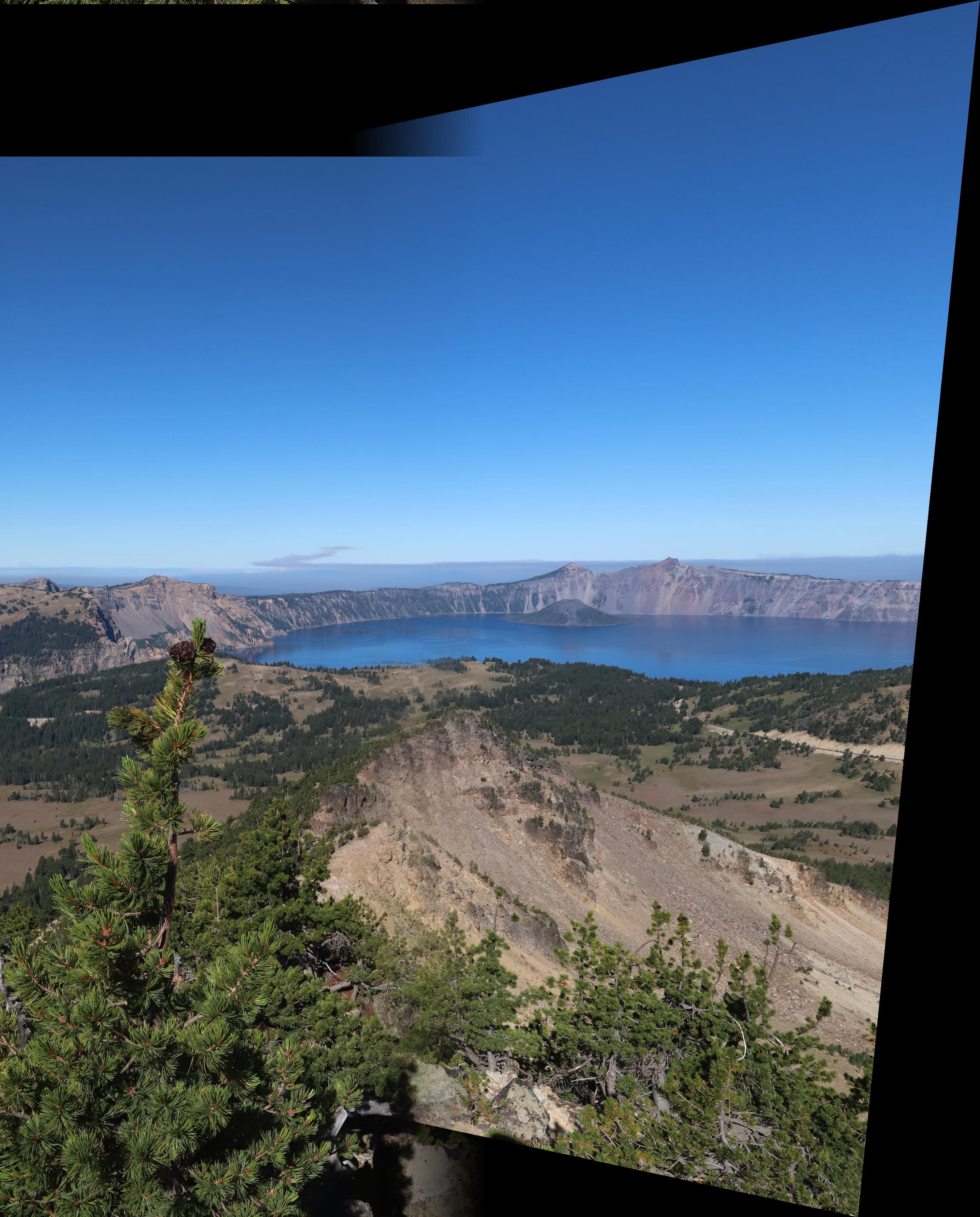
Below are some examples of using my code to generate mosaics automatically. I used some of the same images as above for the sake of comparison. I found that the auto-stitching was cleaner and less error prone, since it didn't require user input for correspondence points.
City
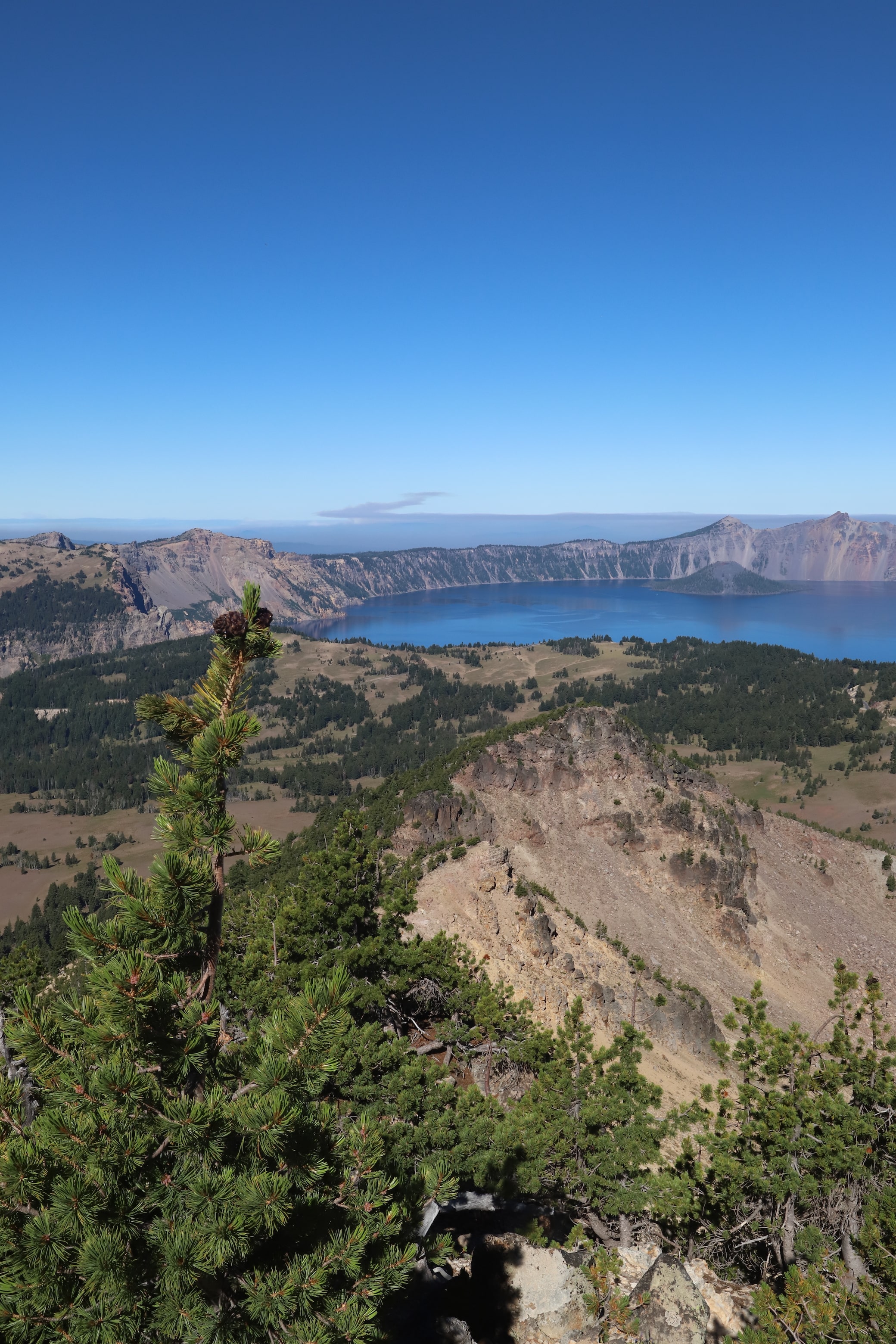
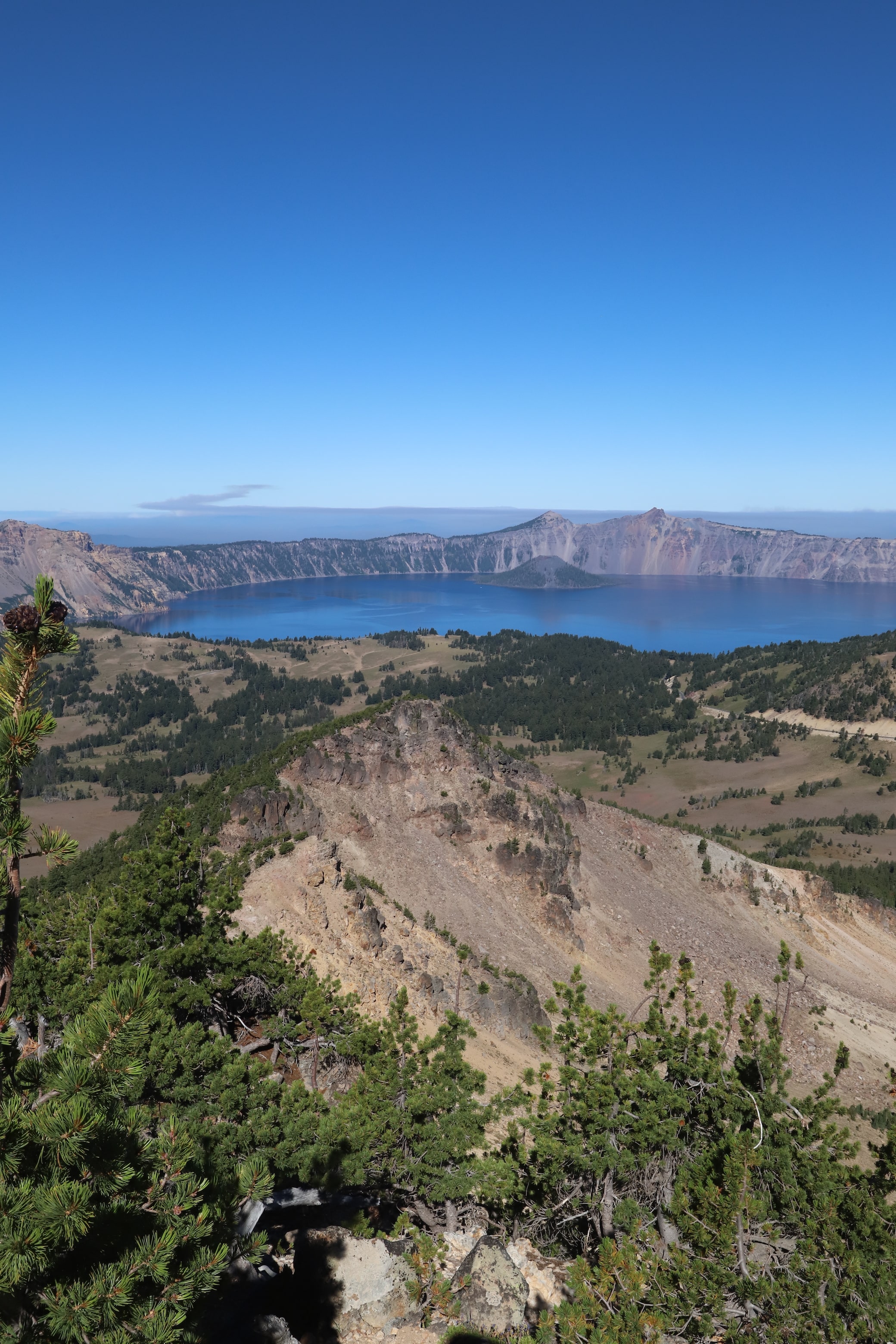
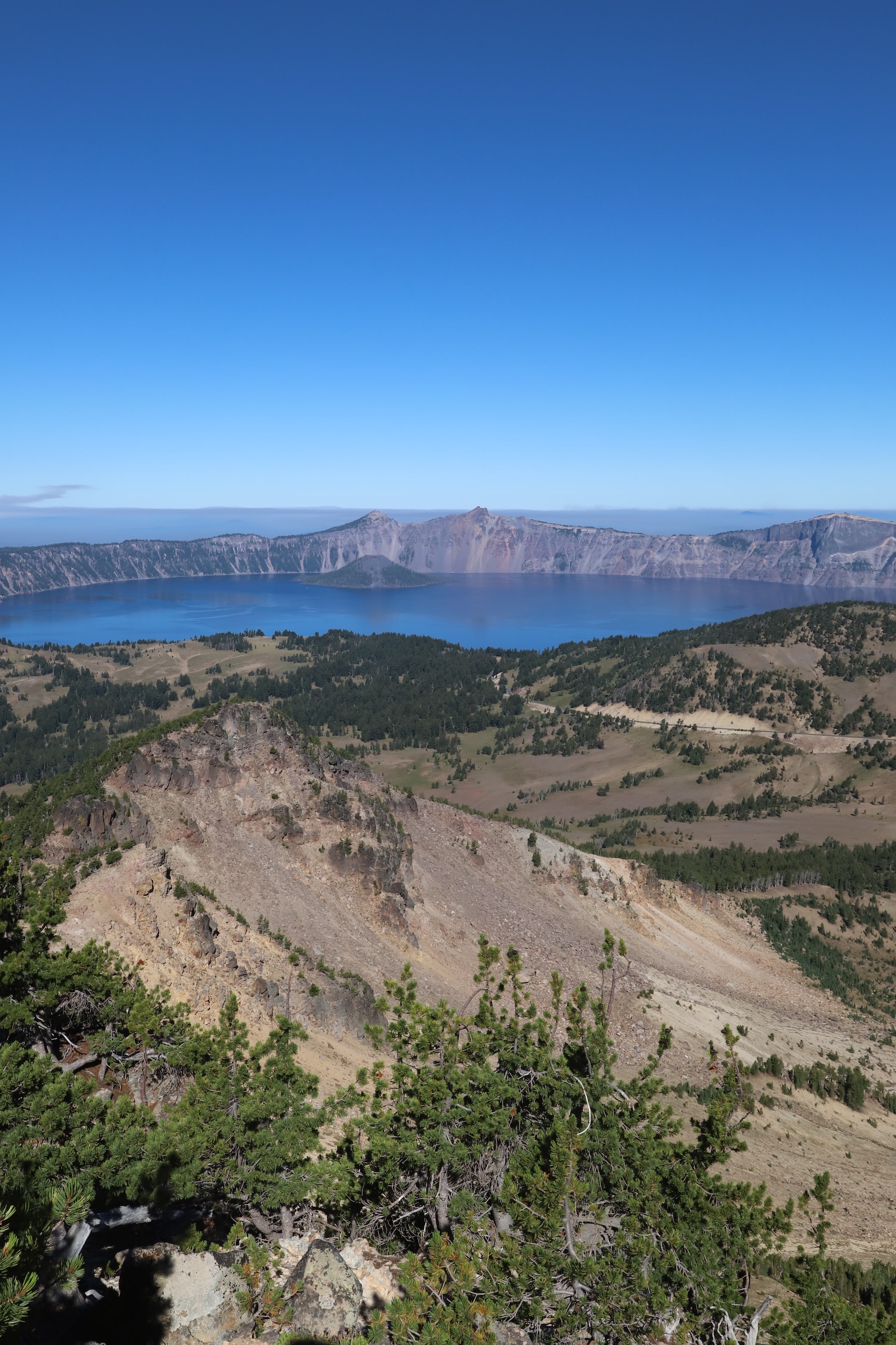
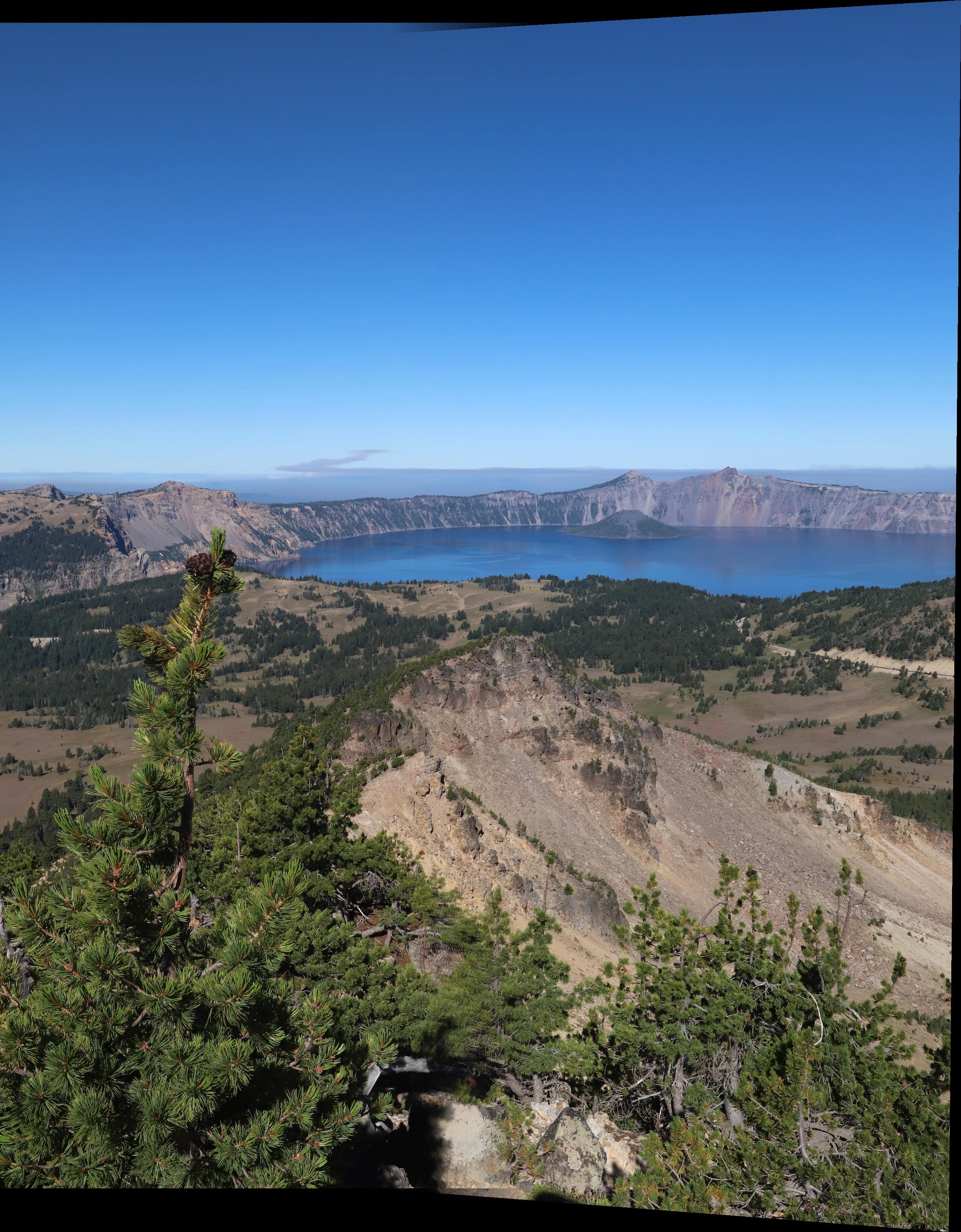
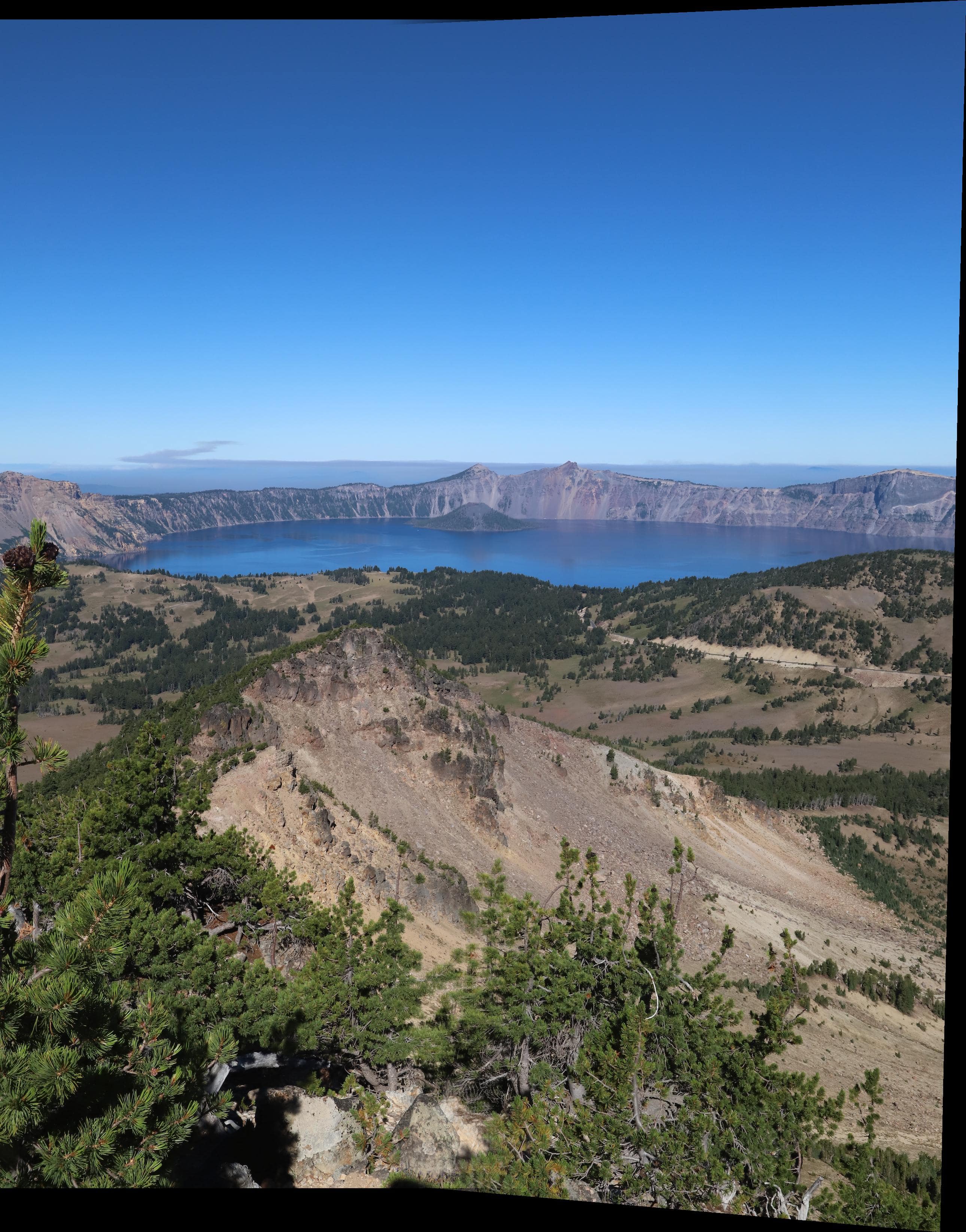
Lake
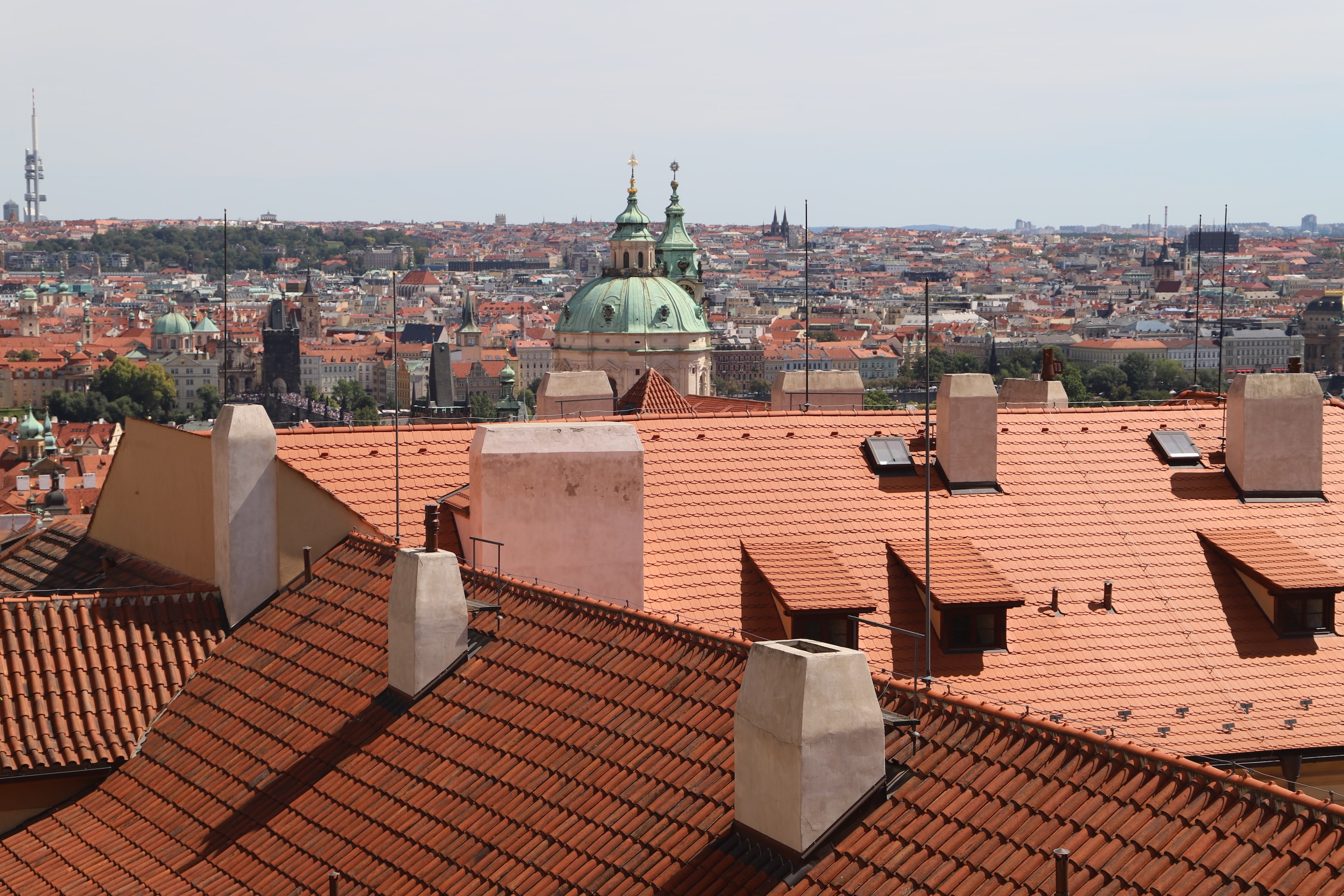
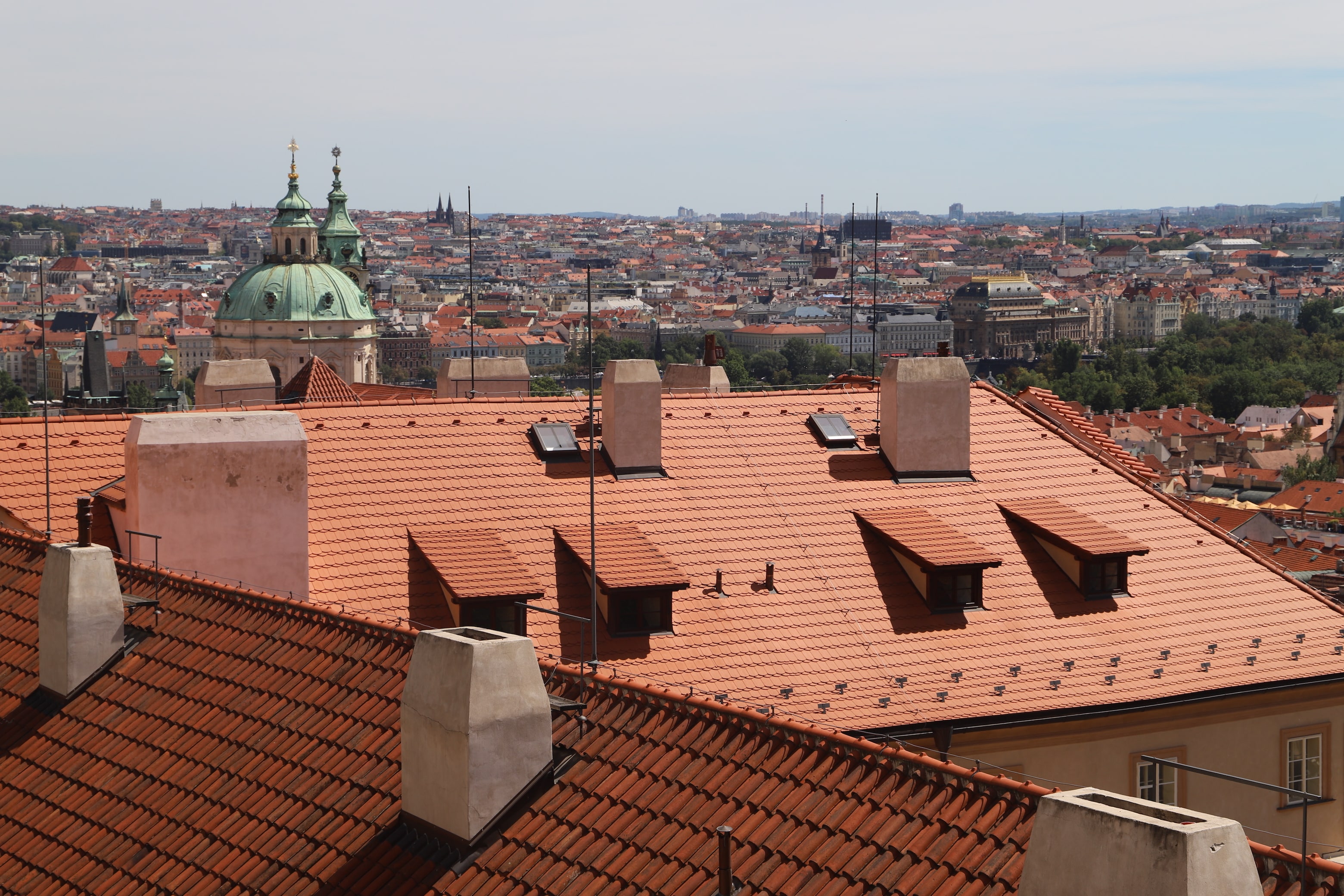
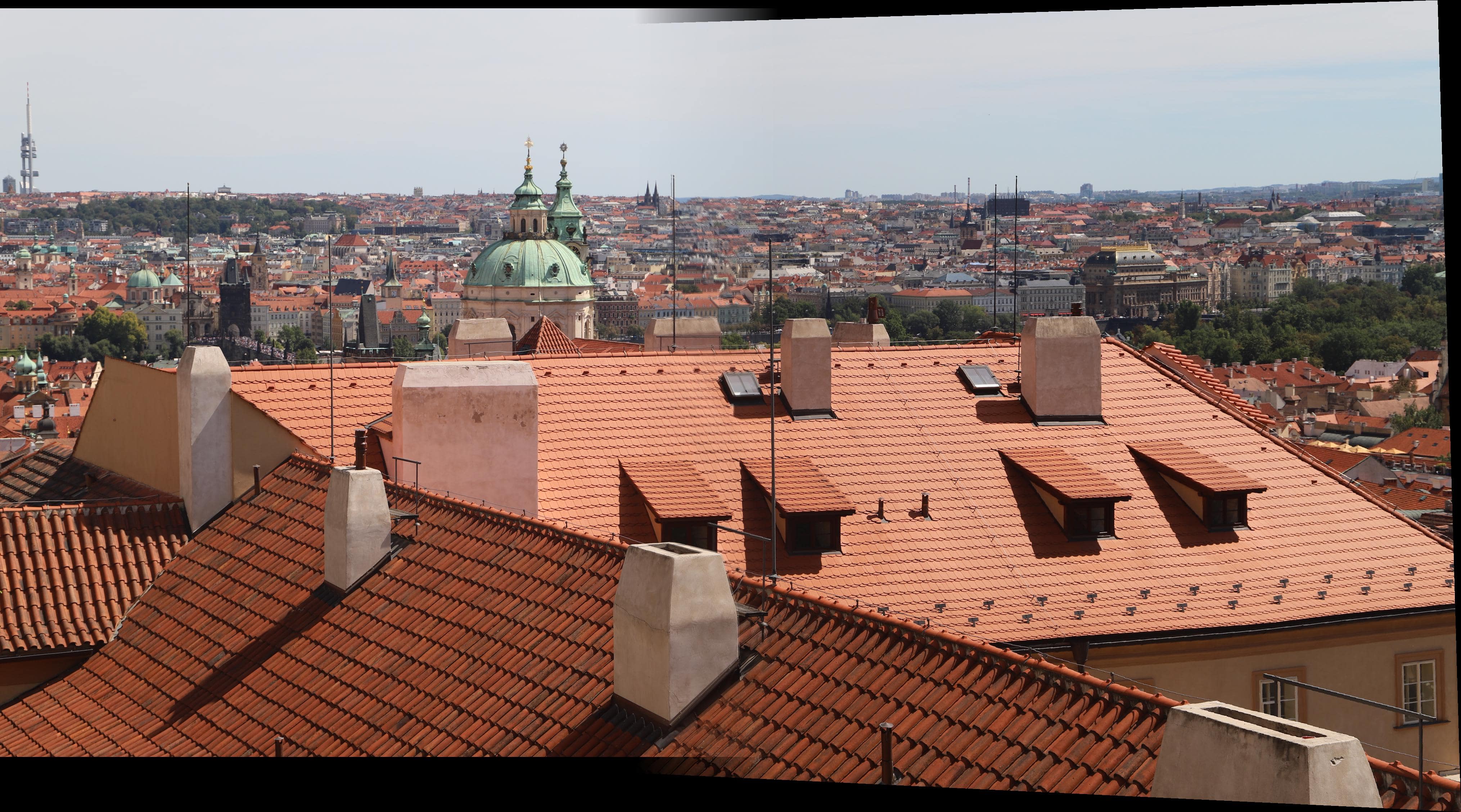
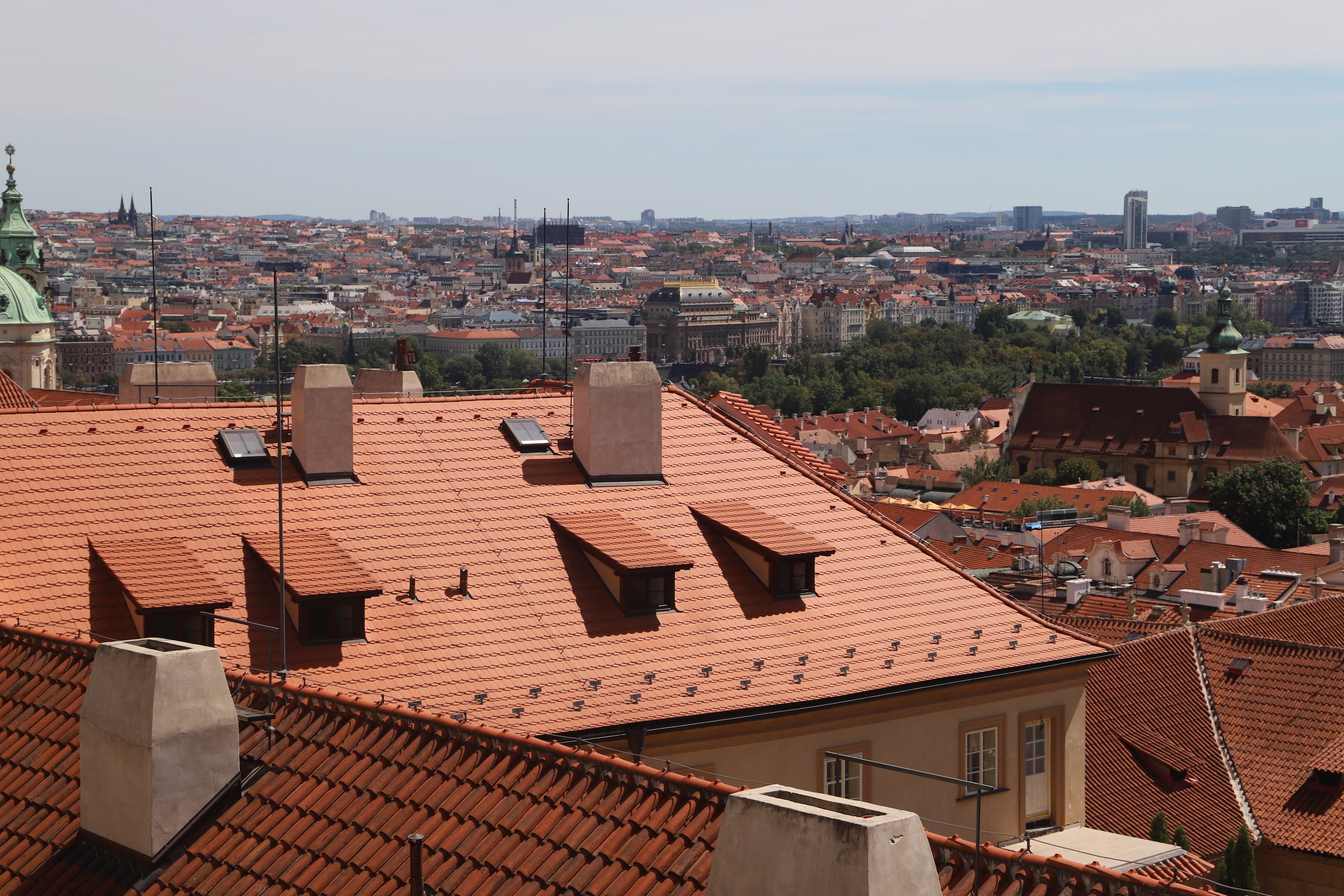
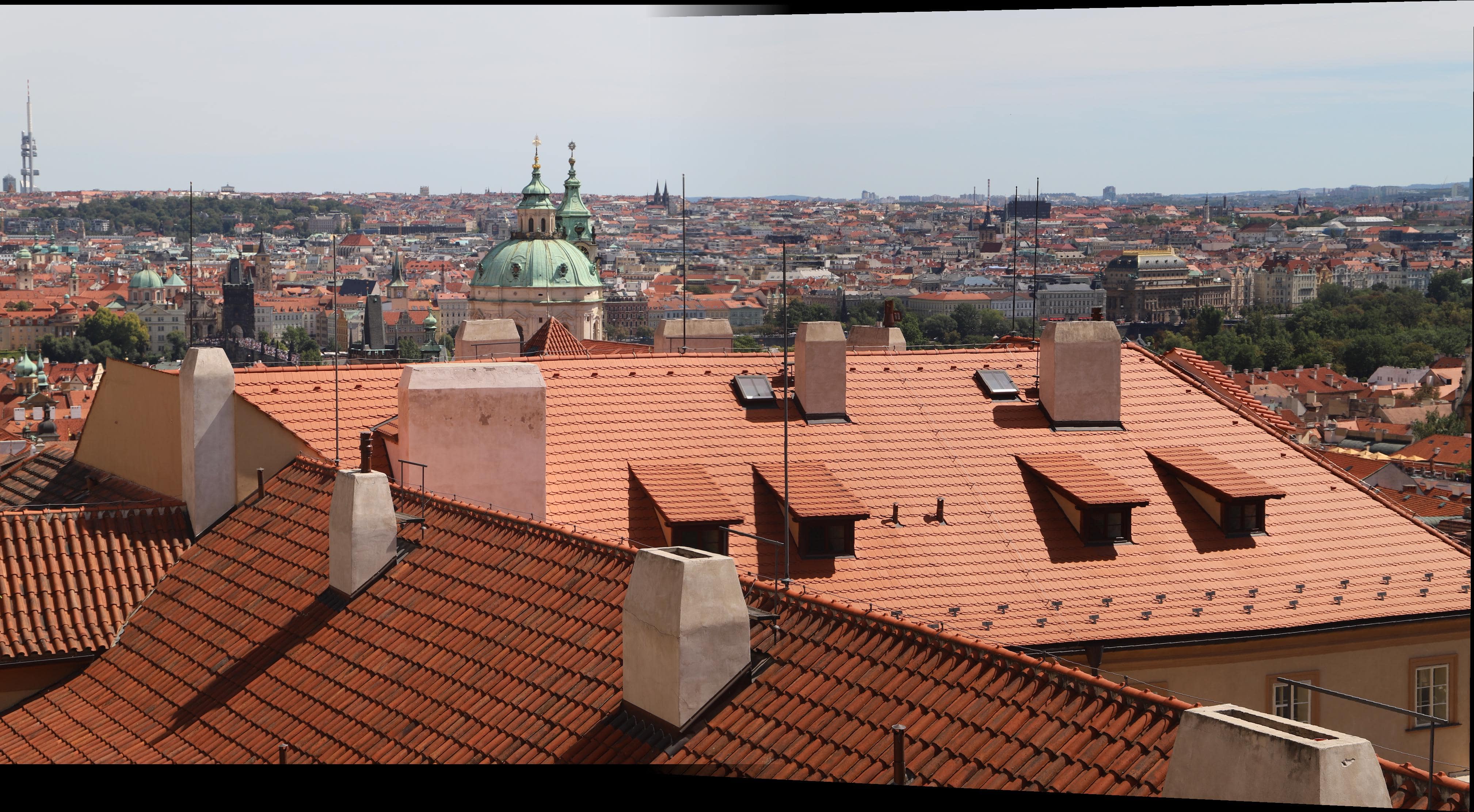
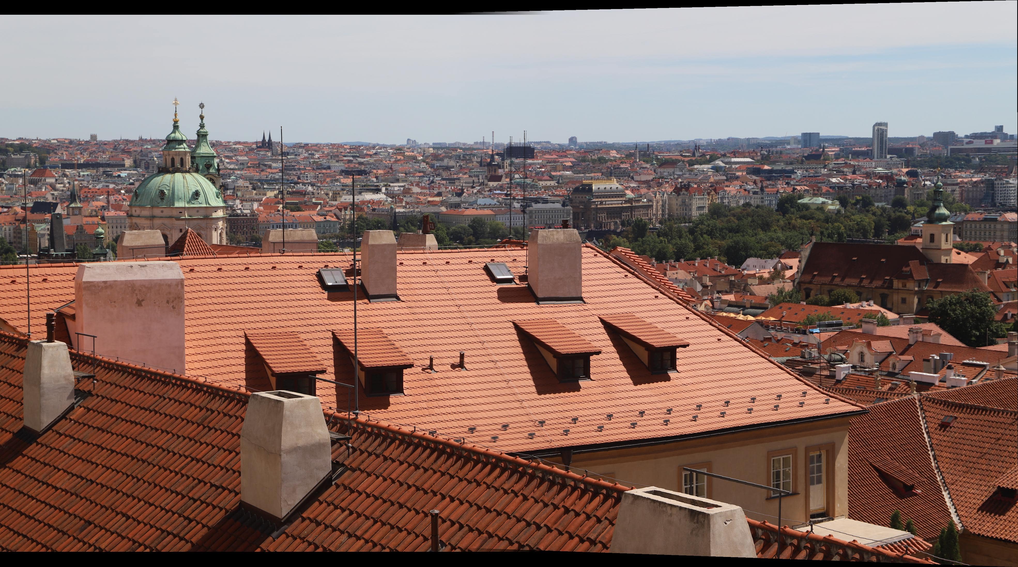
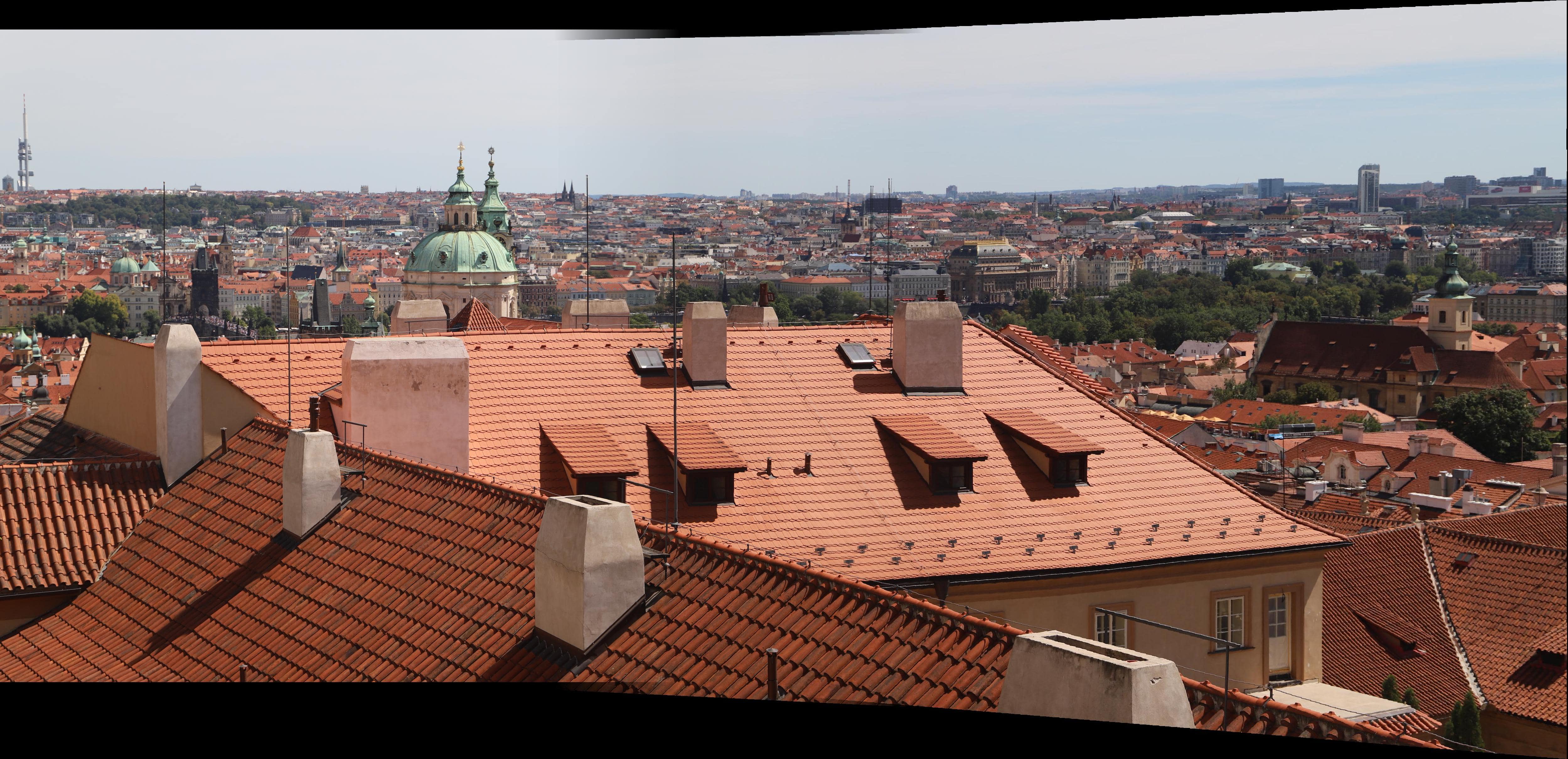
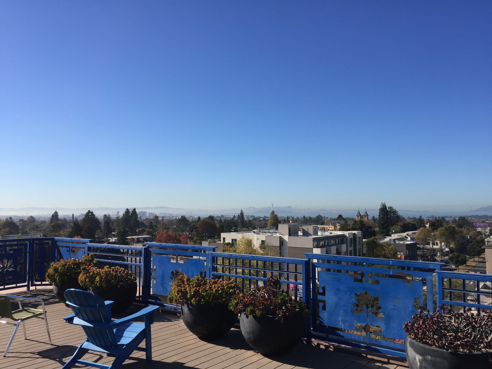
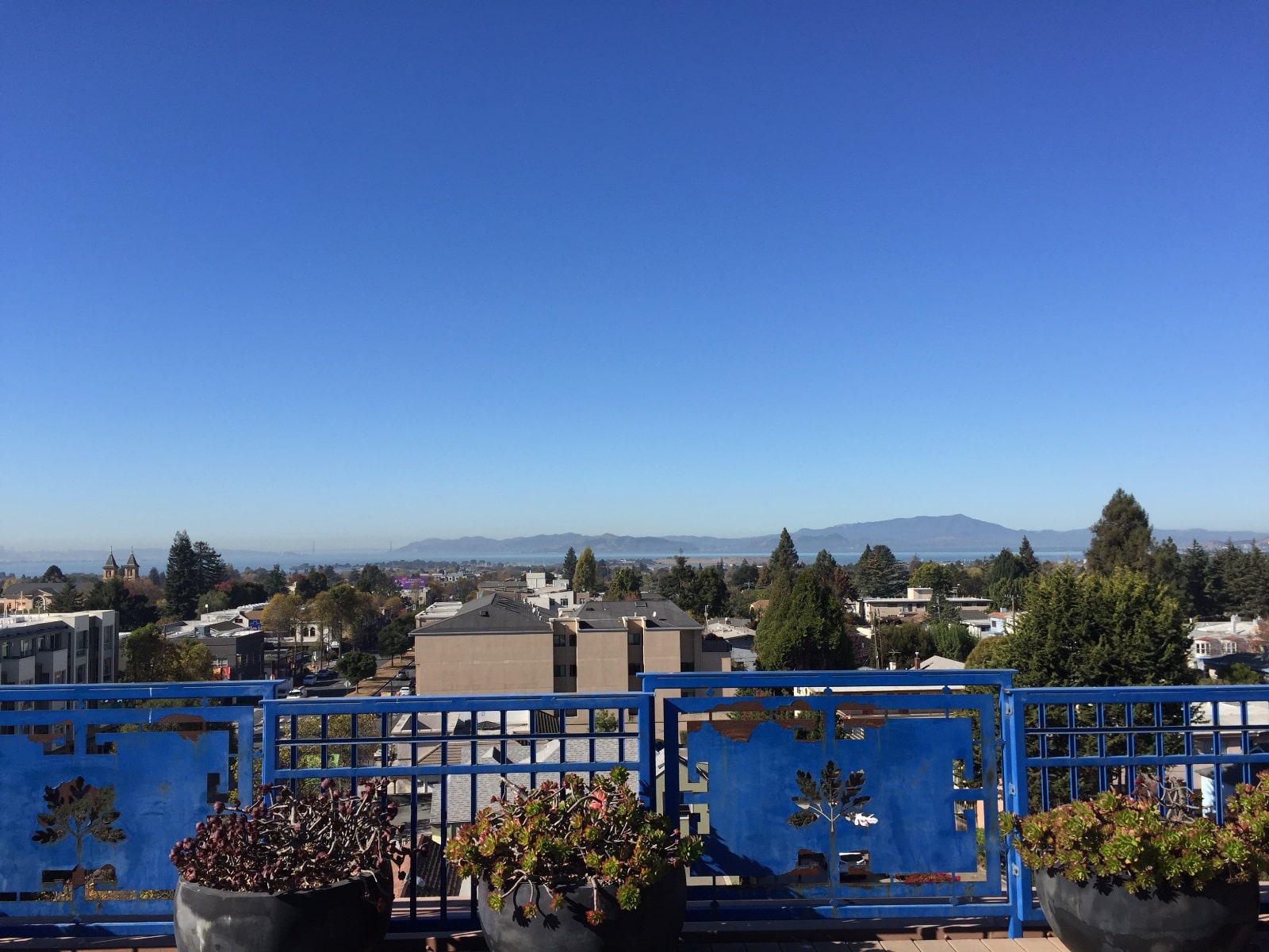
Roof
Images from Andrew Campbell (Fall 18).

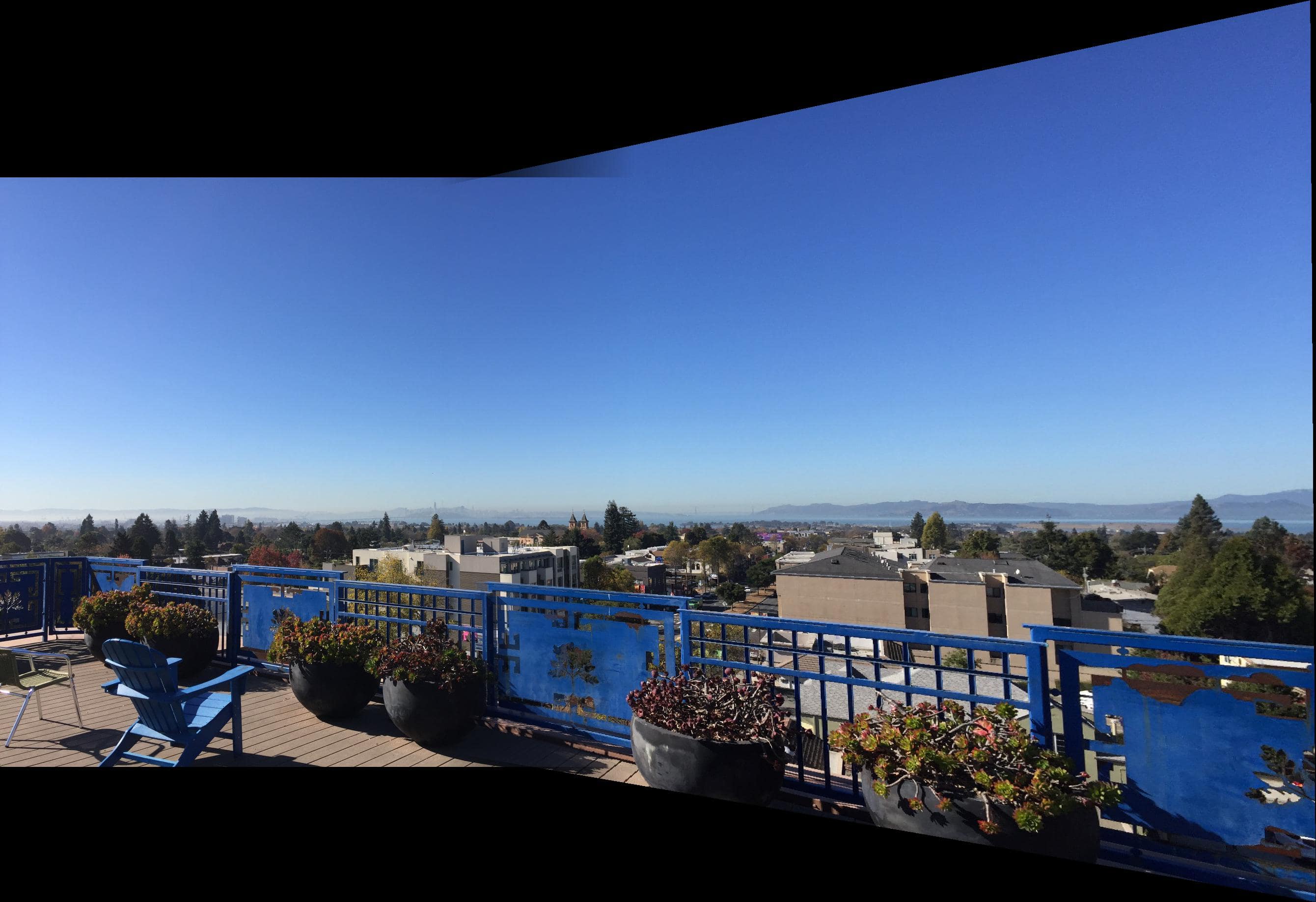
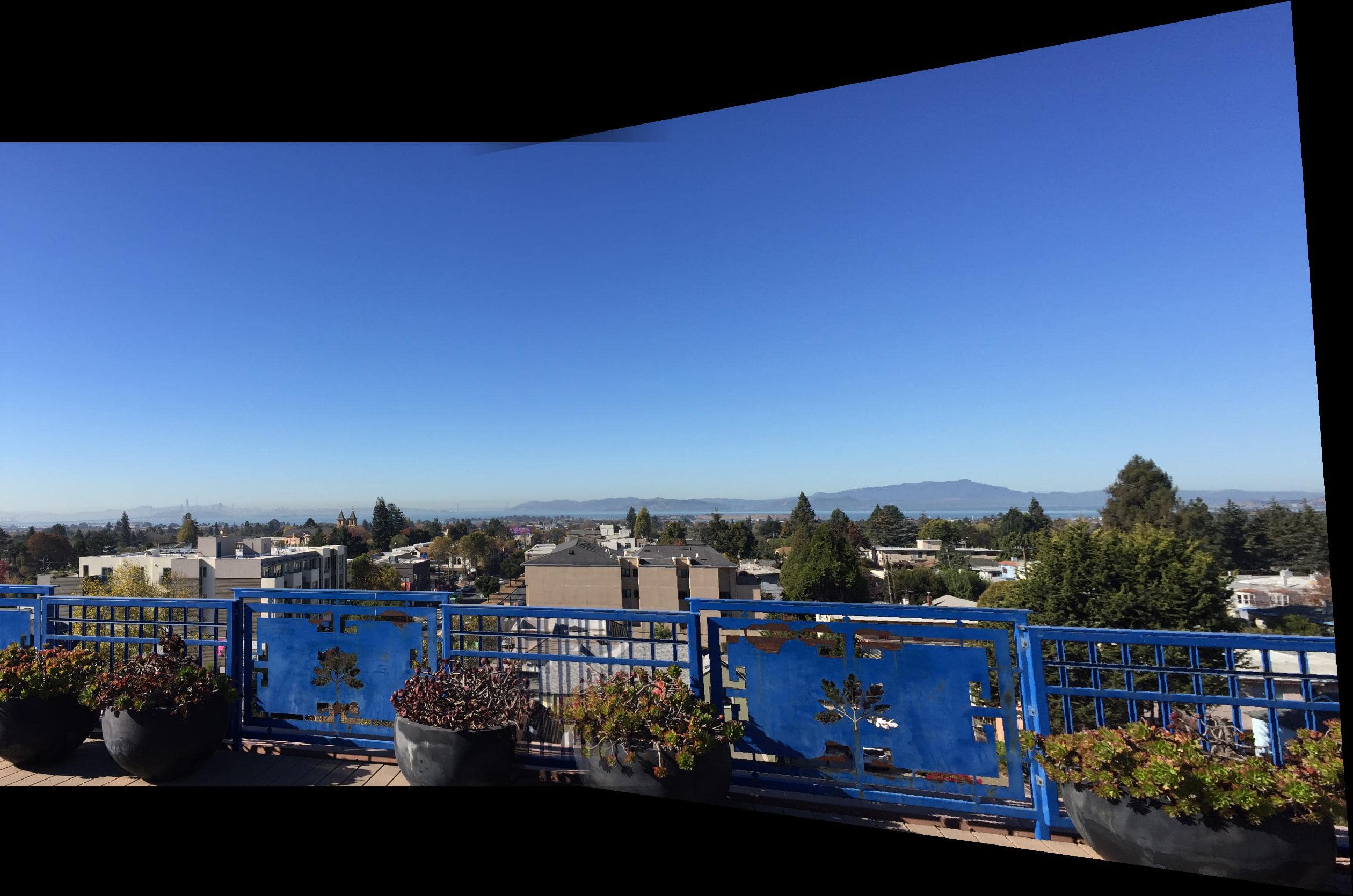
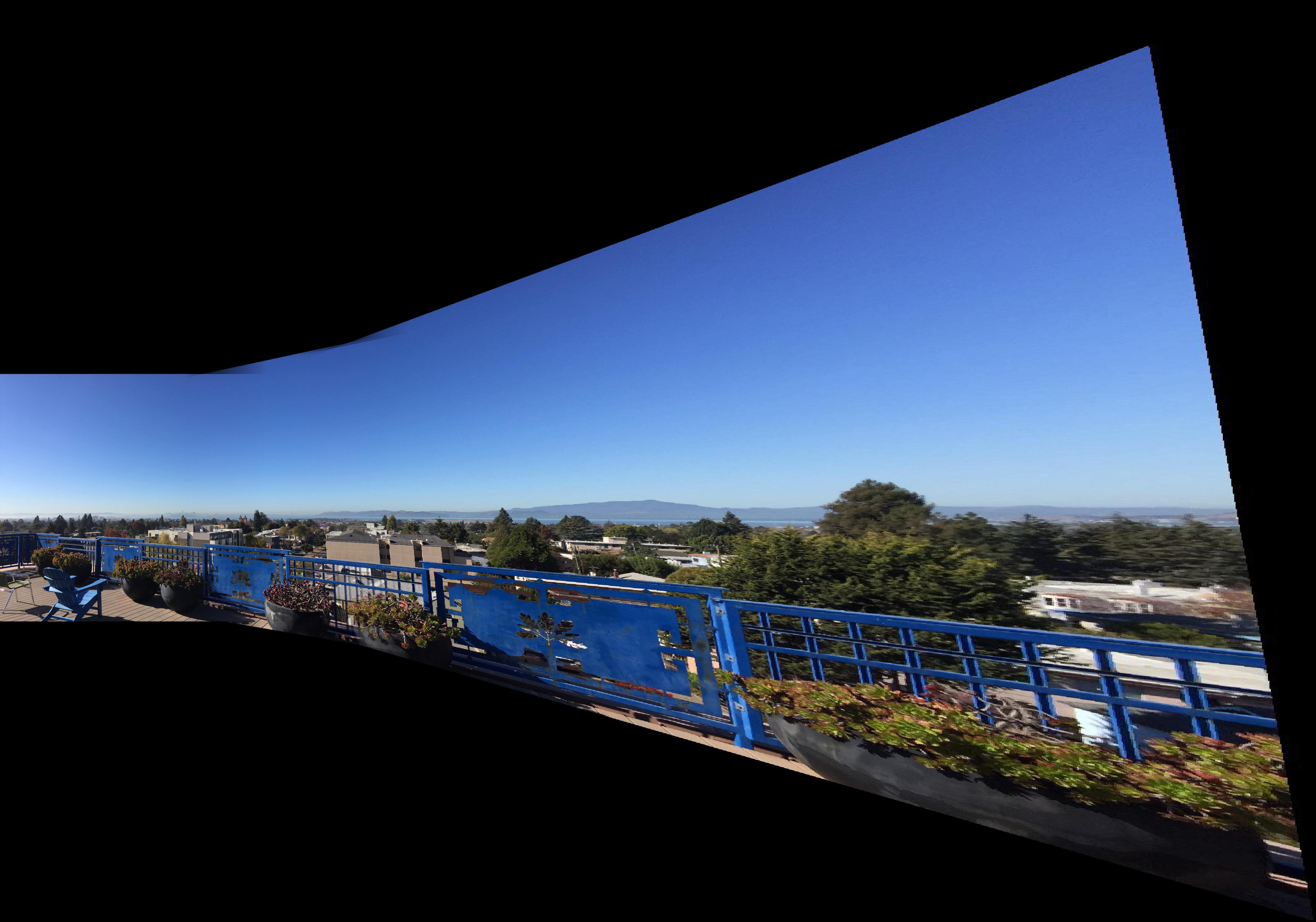
This image produced a lot of warping on the right side. We can see that the images weren't taken properly, since the axis of rotation was not under the lens itself. It was still cool to see the way my code handled this case and put out its best output. Also, since the input image size was smaller than the rest, I had to adjust the min_distance parameter to a lower number when getting Harris corners such that the algorithm had enough points to consider when matching.
Interestingly enough, I found that the implementation of Part 2 was much more intuitive than Part 1. Most of the issues I had with Part 2 were simply solved through discussion with my peers.
Conclusion
Although a lot of this project was quite tedious, I still enjoyed it more than some of the other projects. I found that Part 2 was very interesting and it was nice to see results pop up on my screen. The process of RANSAC is quite simple, but quite effective. I think auto-selecting correspondence points in two images was the coolest thing I learned about in this project. The feature matching portion of the code was most interesting to me.