[Auto]Stitching Photo Mosaics
We can form an image mosaic or panorama by taking multiple overlapping photos from the same point of view and combining them. To align these images properly, we need to warp them using perspective projection onto the same plane, requiring us to first recover homographies between the images that allow us to perform the perspective projection. Warping images allow us to "rectify" them, transforming surfaces in the image that are not frontal-parallel to be so. Once we've successfully warped the images onto the same projective plane, we can blend them together using alpha blending.
Part 1: IMAGE WARPING and MOSAICING
Overview
Recovering Homographies
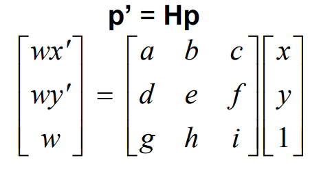
A homography is a perspective projection between two projective planes with the same center of projection. Finding a homography in this scenario requires finding a 3x3 perspective projection, i.e. finding 8 unknown variables in matrix H such that p' = Hp. p and p' in this case are
correspondences between the two images/projective planes.
Given 4 or more correspondences (4 p and p') between the two
images, we can use least squares to solve for the 8 unknowns
a, b, c, d, e, f, g, h (we set i = 1). We solve the equation on the
right to be equivalent to 0 to get the A and b in Ah = b, and run
numpy.linalg.lstsqto get h, giving us the 8 unknowns.
Once we have H, we can use it to warp from coordinates in one
image into coordinates for another image. We normalize these output coordinates so that w = 1 as in the input coordinates.
Warping Images
To warp from one image A to another image B, we first recover the homography/perspective projection from A to B. We then use inverse warping from A to B by first calculating the inverse of H, and then for every coordinate in B applying this inverse H onto it to get the corresponding coordinate in A. Note that these output coordinates in A will be float instead of integer, so we use linear interpolation to get the pixel value to reduce aliasing in the output image. In this case, I used scipy.interpolate.RegularGridInterpolator.
Image Rectification
We can see image warping in action by performing rectification on some images. This transforms parts of images that are not frontal-parallel to appear to be on a frontal-parallel plane. Here we simply need 4 correspondences (where the points in the output form a rectangle) to get a good looking rectification. Below are a few examples of rectification of floor tiles, wall art, and a laptop screen.

Original Image

Rectified Image


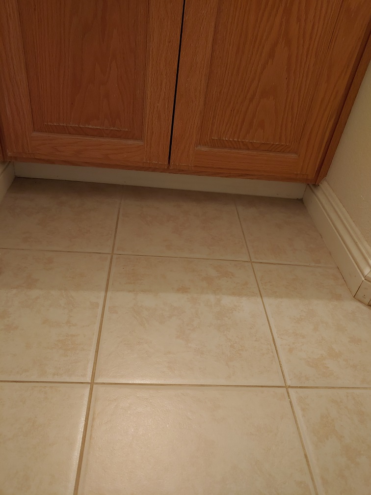
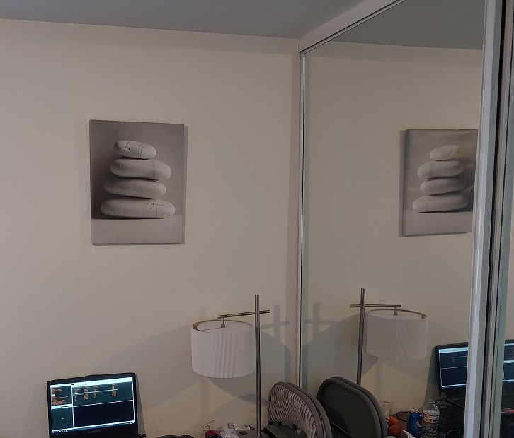
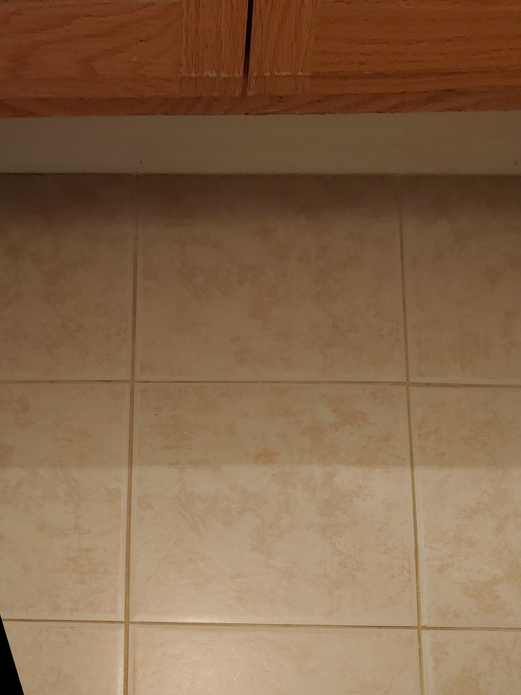
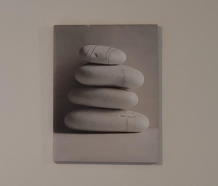
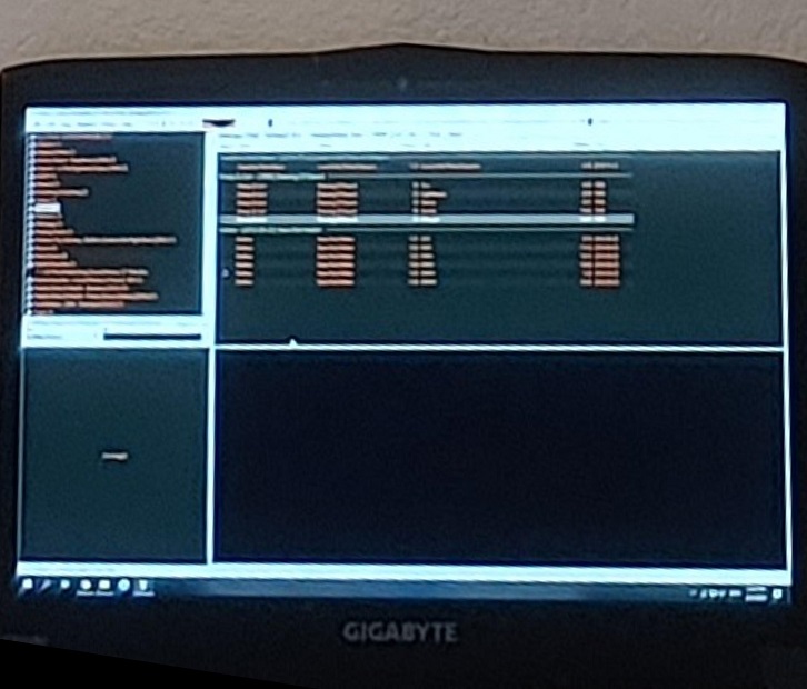
Image Mosaic
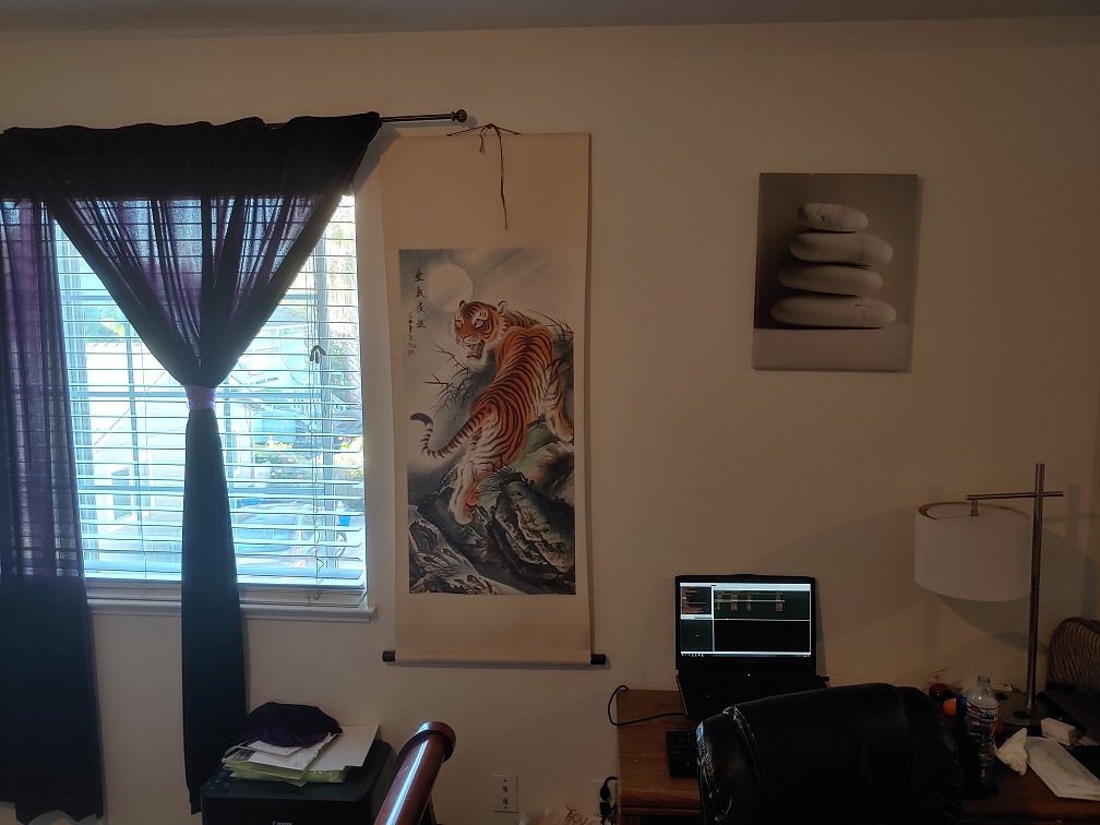
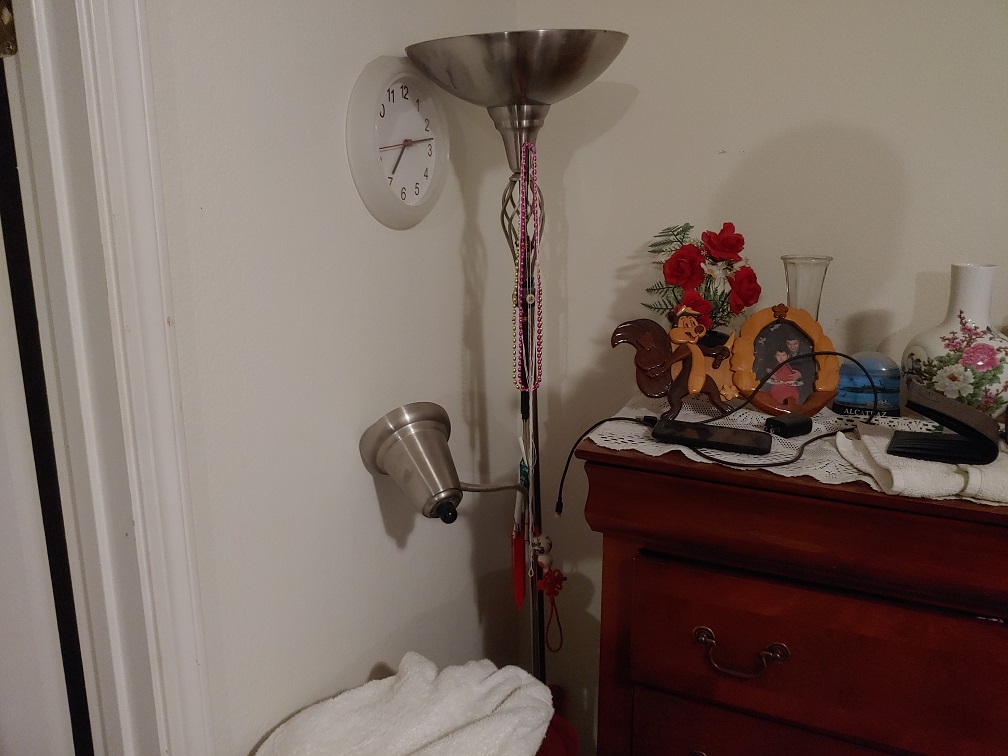
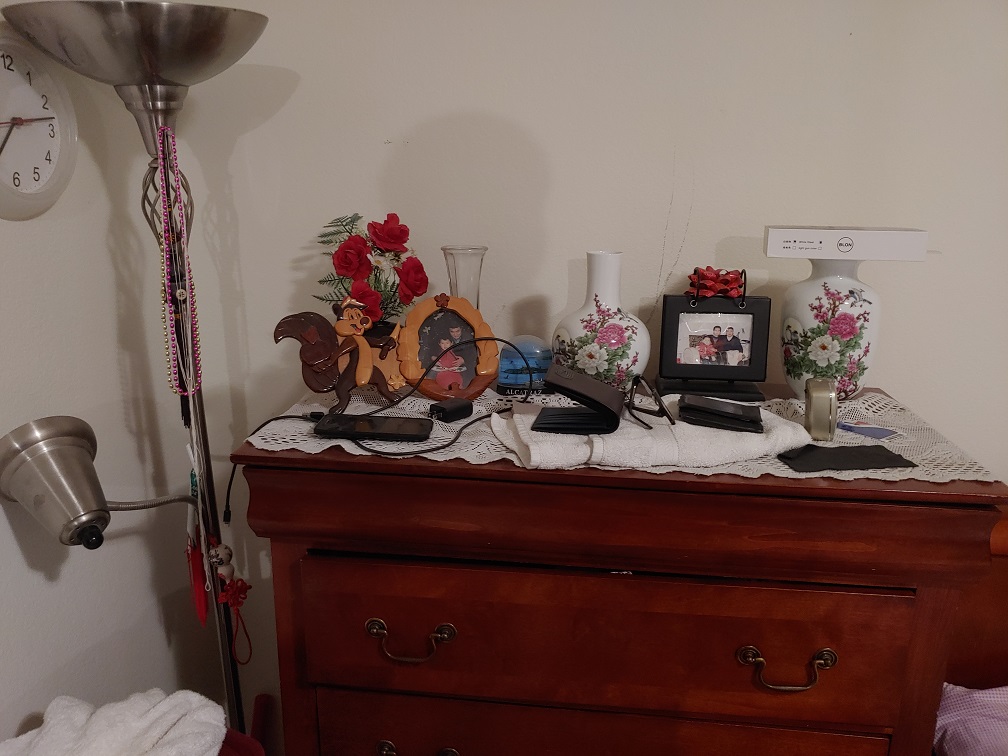
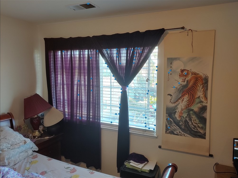
For my image mosaic, I took three pictures (A, B, C) of my room. To blend them together, I first put the middle picture (B) into a large enough canvas to contain all three images (call this B'). I make sure to offset the points selected for B so that they are accurate for B'. Then I computed homographies from the left picture (A) to B' and from the right picture (C) to B'. From there I simply inverse warp from A and C to B'. To avoid edges in the blending, I applied alpha masks to each image, using simple linear fall off of values from the center. Below shows pictures I took in my room and the mosaics I created out of them.


Part 1 Conclusion
This part helped me a lot with understanding how projective projection works and how it can be calculated easily using a set of correspondences and least squares. I was also surprised by how good the rectifications and mosaic looked. Given a high enough resolution starting image and linear interpolation, the rectifications look like they're completely separate photos taken from a different angle rather than a transformation of the original image, and I loved how that effect could be accomplished with just a simple perspective projection.
Part 2: FEATURE MATCHING for AUTOSTITCHING
Detecting Corner Features In An Image
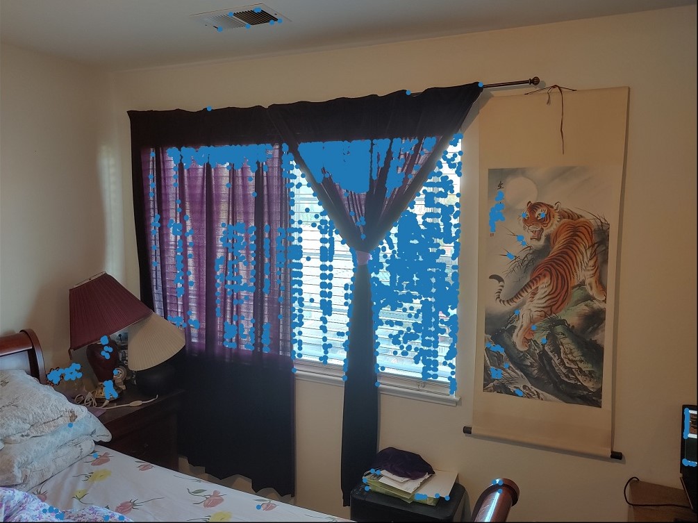
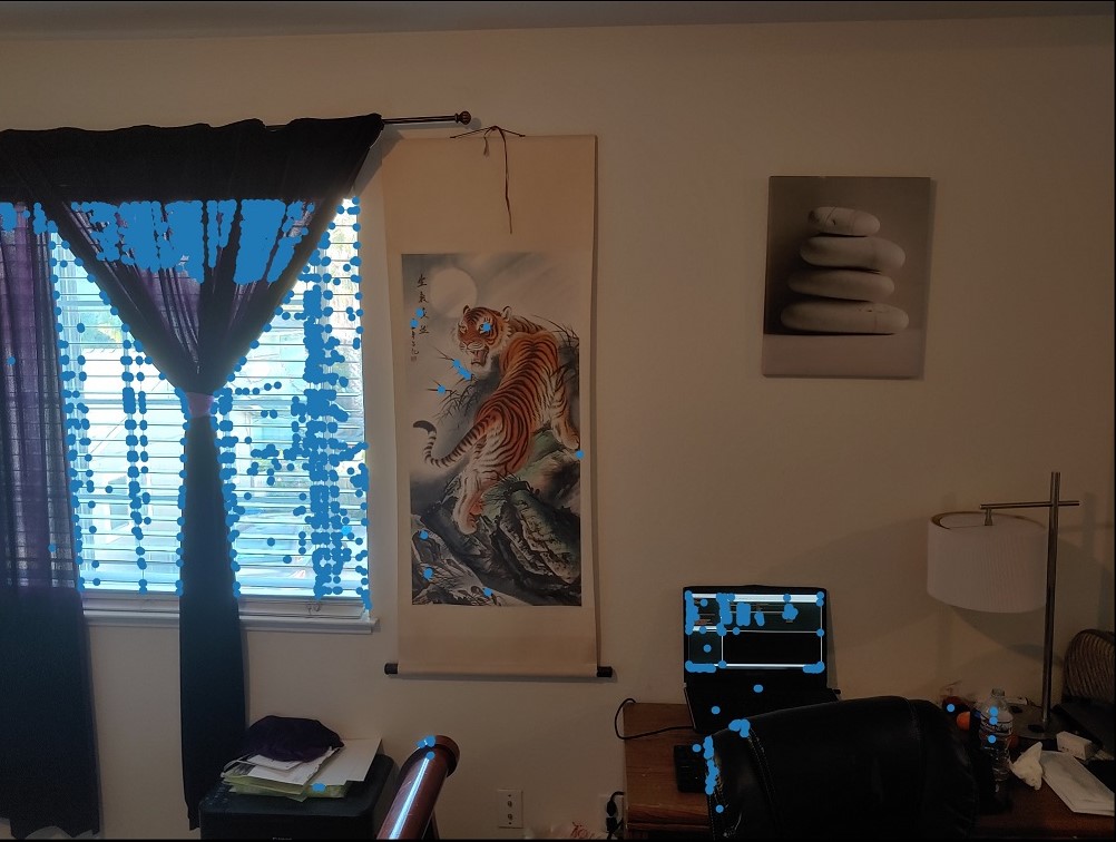
We perform feature detection using Harris corners, which is based on changes in intensity due to shifting a window in any direction. Thus, locations with significant change in all directions likely correspond with a corner in the image. Below shows the detected Harris corners on some images (blue dots).
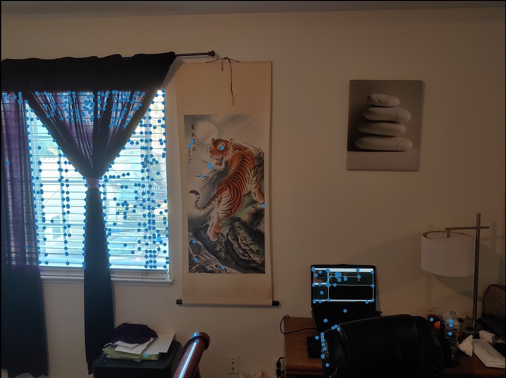
Since we want our chosen points to be limited in number and also spread apart evenly, we use Adaptive Non-Maximal Suppression: for each point i detected by Harris corners, we calculate its minimum suppression radius:
We then keep the 500 points with the largest minimum suppression radiuses. The remaining points have strong corner strength but are also spread apart evenly:


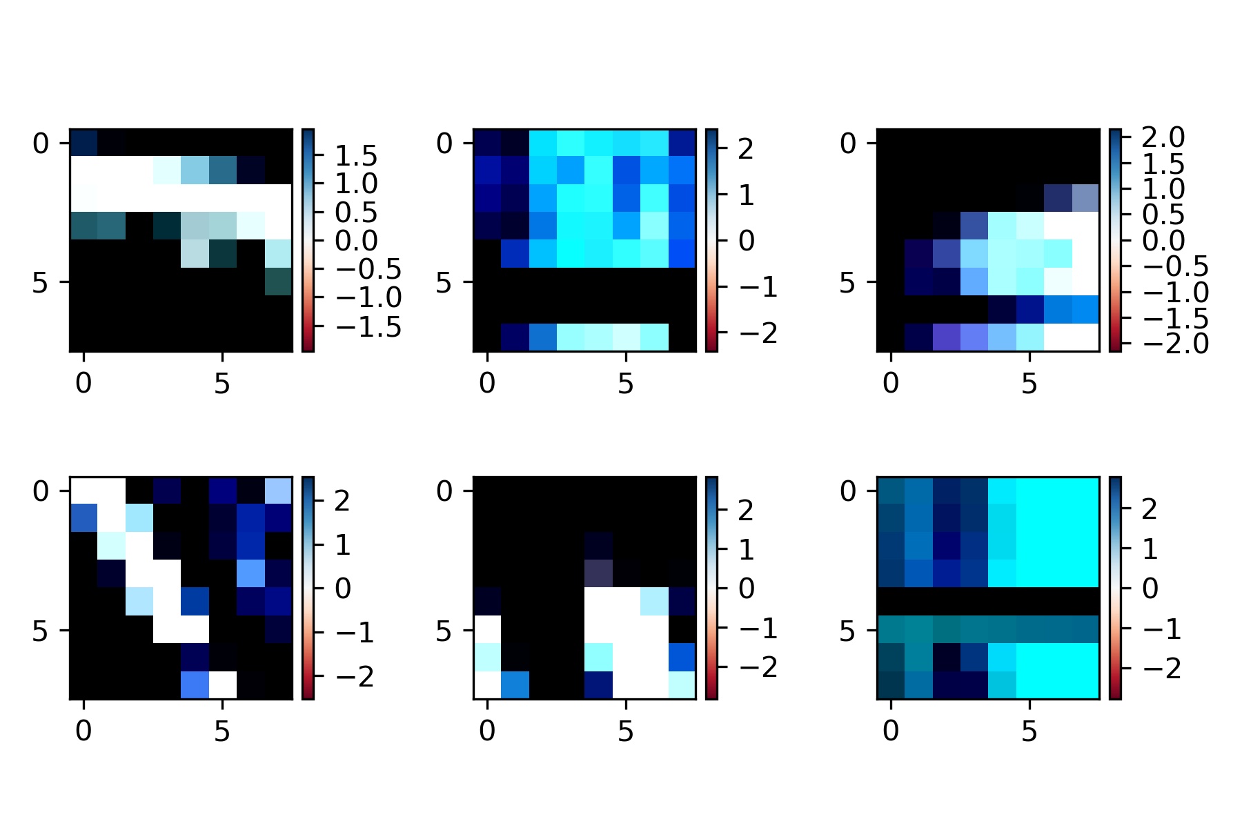
Extracting A Feature Descriptor For Each Feature Point
To get a feature descriptor for a feature point, we sample a 40x40 patch around the point in the image, downsampling to an 8x8 patch and then performing bias and gain normalization on it. Below shows some feature descriptors for the left image above.
Matching Feature Descriptors Between Two Images
We use the sum of squared distances (SSD) to compare feature descriptors between two images to find pairs. For each feature descriptor in the first image, we compare it with each feature descriptor in the second image. We get the closest match (1-NN) and second closest match (2-NN) and calculate the ratio 1-NN/2-NN, accepting the pair only if that ratio is below some threshold (Lowe Thresholding). This is so that our match is actually much closer to the feature descriptor than other close matches, and not just one match out of many similar matches in which case it's likely incorrect. Below shows some results of this feature matching.

Using RANSAC To Compute A Homography
You can see in the above two images that while most pairs of points match properly (inliers), there are some correspondences that don't match properly (outliers). We need to remove these by performing outlier rejection using RANSAC (Random Sample Consensus). In a loop, we select 4 feature pairs at random, compute the homography, and use this homography to warp all points from the first image. We then compare these warped points to the second image's points, and keep only pairs where the SSD between the points are less than a certain threshold. I found a threshold of 0.5 and 10,000 loops to be effective while not taking too long. This results in all outliers being rejected, but also results in far fewer matches since each calculated homography in RANSAC is based on only 4 points.
Below shows RANSAC matches between two images.
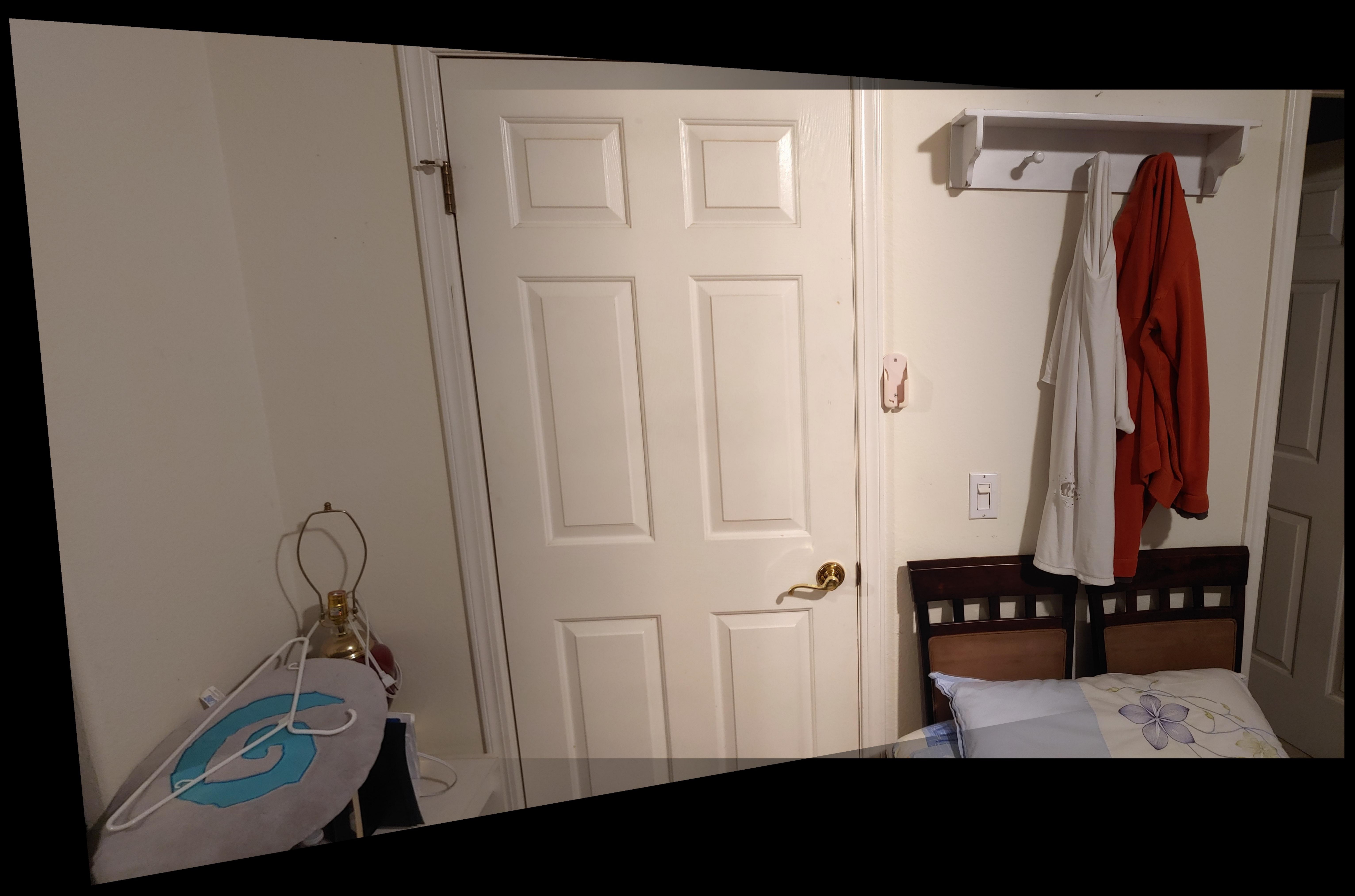
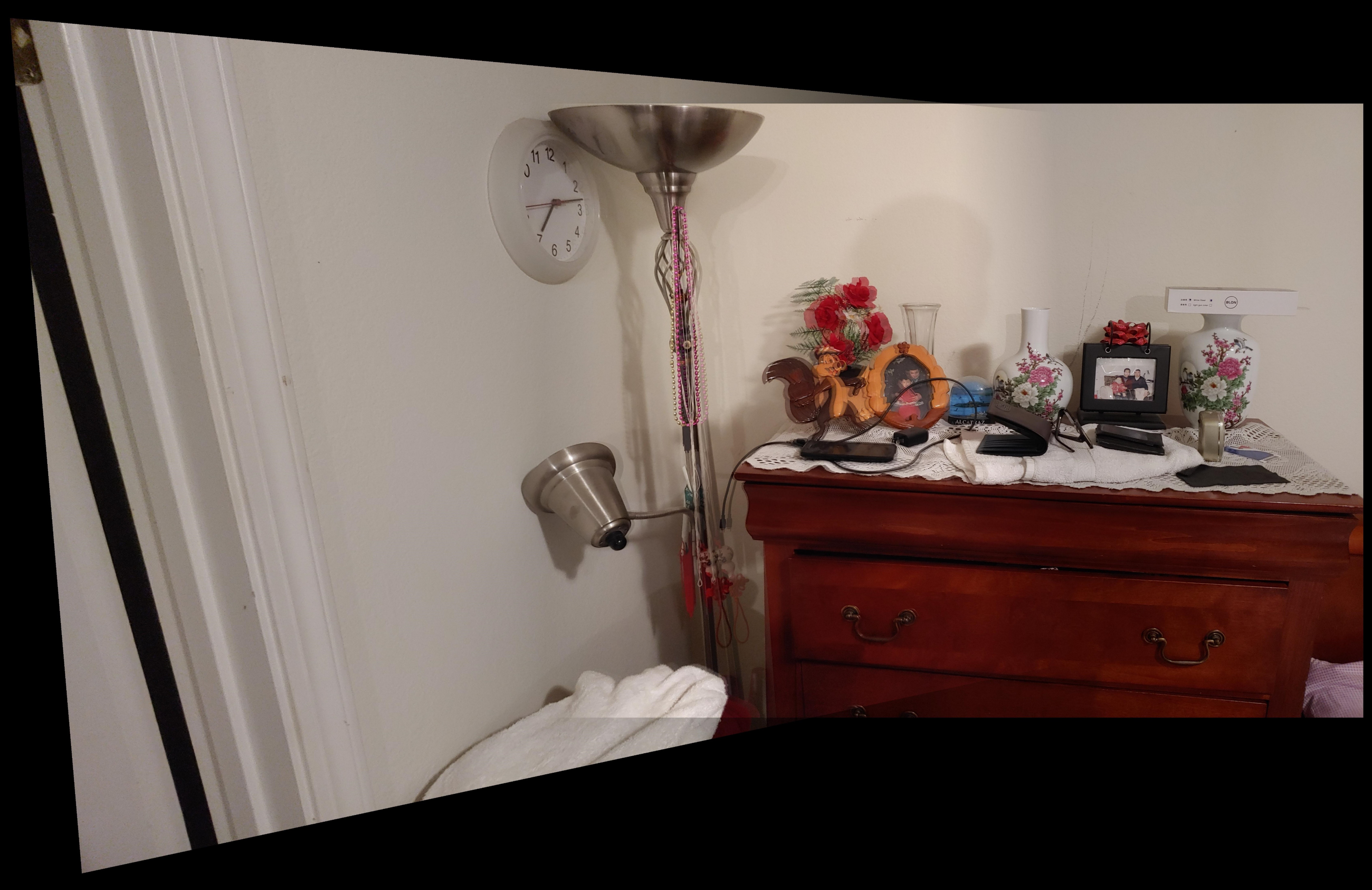
Below we show the manually selected feature mosaics from part 1 compared to the automatically feature matched mosaics from this part (manual image on top, automatic image below).
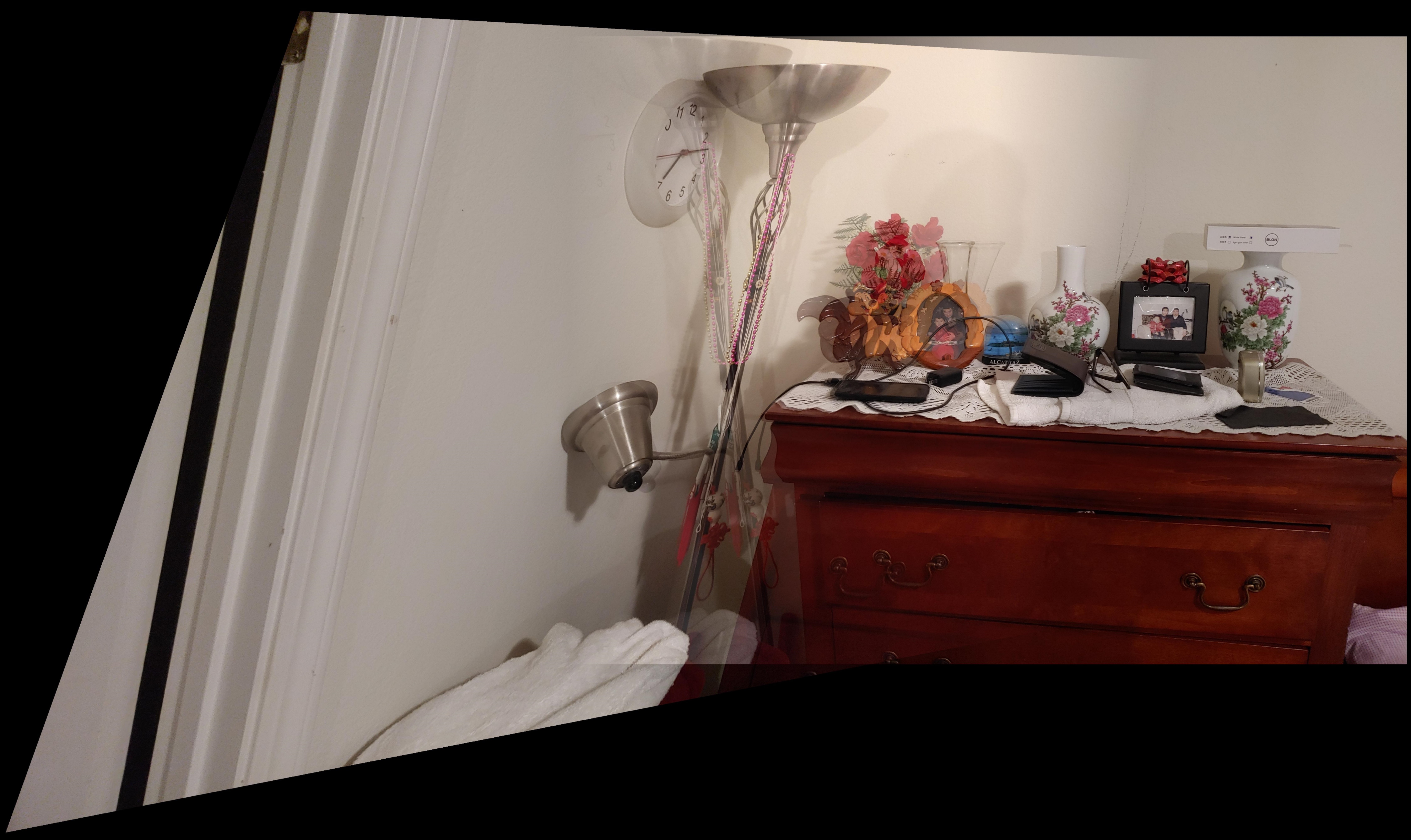
This example was particularly striking since the calculated homography in the automatic feature matching image was very off compared to the manual image. This is because the matched pairs of points were all in the middle of the image on the table. This meant that while the middle of the image looks okay, the homography transformation neglected to account for the tall lamp on the left, causing a very shifted shearing look on the left side of the image. I tried to raise the number of RANSAC loops to 50,000 and also increased the threshold to try to get some correspondences on the lamp, but was unsuccessful. This is probably because there's such a discrepancy between how the lamp looks transformed vs how the table looks transformed when using a 4-point homography during RANSAC.
Part 2 Conclusion
I really enjoyed working through this part and seeing how each step remedied some issue from the previous part. It was really cool to get such a robust automatic feature matching algorithm from what seems like a series of ad hoc procedures. I have a better understanding now of Harris corners, ANMS, feature descriptors, and RANSAC. This feature matching algorithm is also surprisingly fast and can produce results that differ very little from manual feature matching.