Part 1: Image Warping and Mosaicing
Recovering Homographies
Any two images of the same planar surface in space are related by a homography, which can be represented by a homography matrix.
$$H = \begin{bmatrix} a & b & c \\ d & e & f \\ g & h & 1 \end{bmatrix} $$This method technically only requires four point correspondence pairs to be recovered, but in practice, least square regression on many pairs of points works better. $$\begin{bmatrix} x_{1,1} & y_{1,1} & 1 & 0 & 0 & 0 & -x_{1,1} x_{2,1} & -y_{1,1} x_{2,1} \\ 0 & 0 & 0 & x_{1,1} & y_{1,1} & 1 & -x_{1,1} y_{2,1} & -y_{1,1} y_{2,1} \\ & & & & \vdots & & & \\ x_{1,n} & y_{1,n} & 1 & 0 & 0 & 0 & -x_{1,n} x_{2,n} & -y_{1,n} x_{2,n} \\ 0 & 0 & 0 & x_{1,n} & y_{1,n} & 1 & -x_{1,n} y_{2,n} & -y_{1,n} y_{2,n} \\ \end{bmatrix} \begin{bmatrix} a \\ b \\ c \\ d \\ e \\ f \\ g \\ h \end{bmatrix} = \begin{bmatrix} x_{2,1} \\ y_{2,1} \\ \vdots \\ x_{2,n} \\ y_{2,n} \end{bmatrix}. %]]> $$
Using the equations above, we can calculate the homography matrix. For this part, point correspondences are manually chosen.
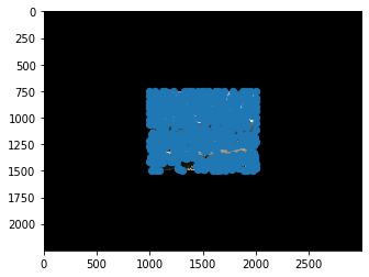
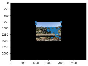
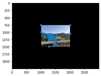
Image Rectification
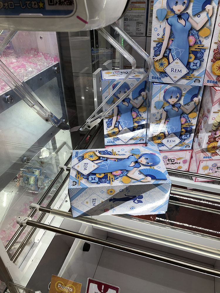
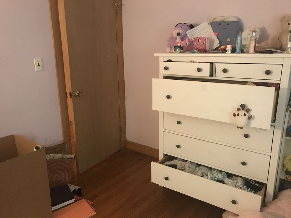
We can now perform (inverse) image warping: for every coordinate value in the output result, multiply by the (inverse) homography matrix, taking care to normalize w to be 1, to recover the coordinates in the original image. One application of a homography is image rectification: given an image containing a planar surface, warp it so that it is frontal-parallel. We simply select 4 points representing the corners of the plane in the original image and choose the correponding points in the output to be the corners of a rectangle. Below we illustrate some examples.


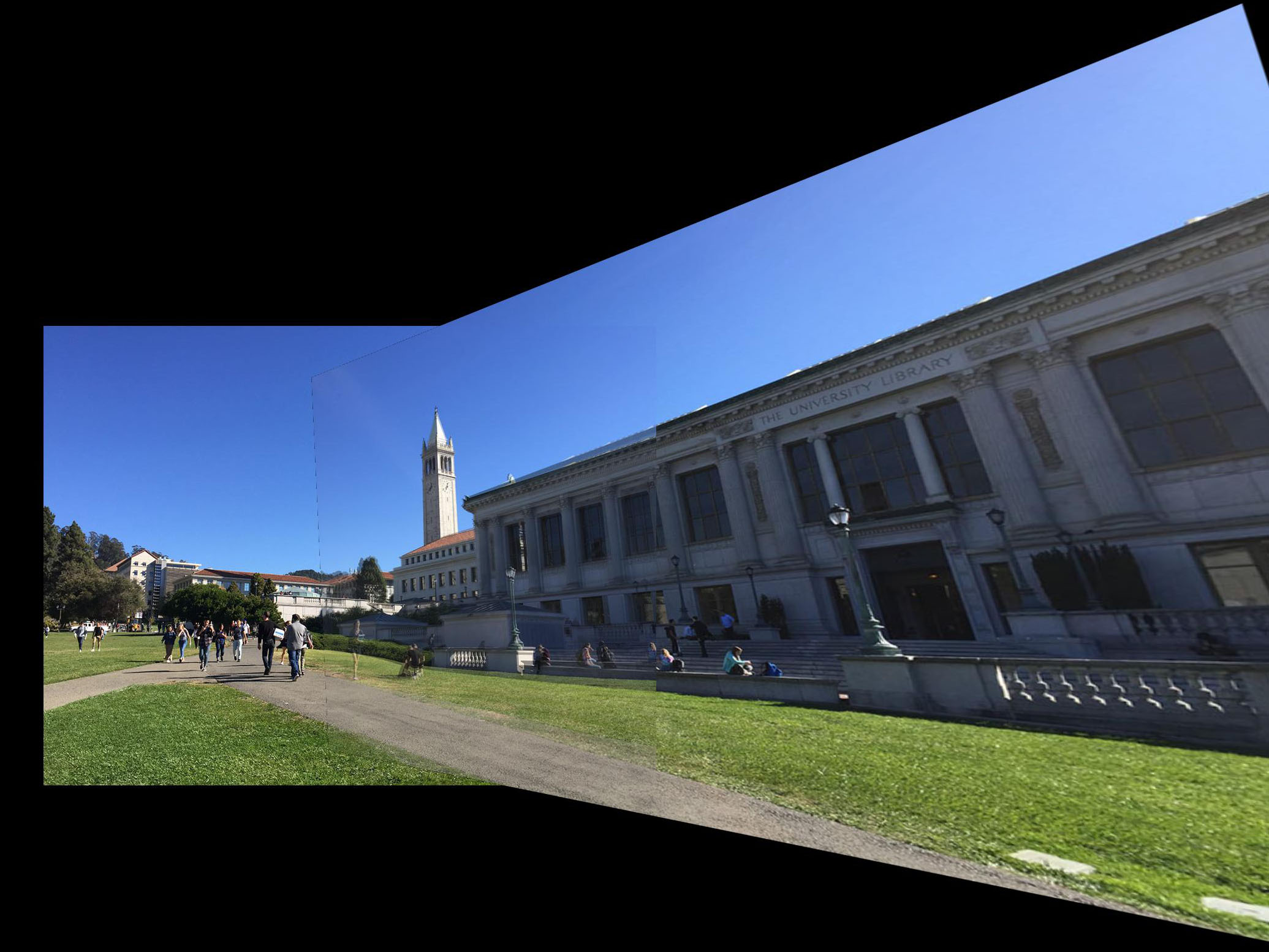
Mosaics
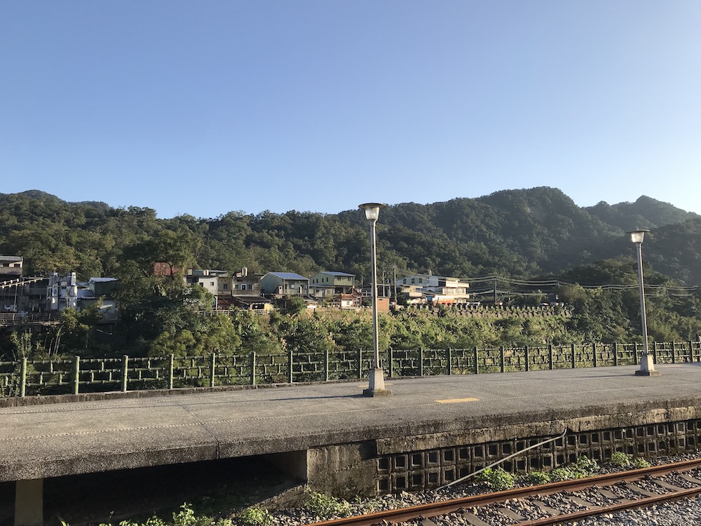
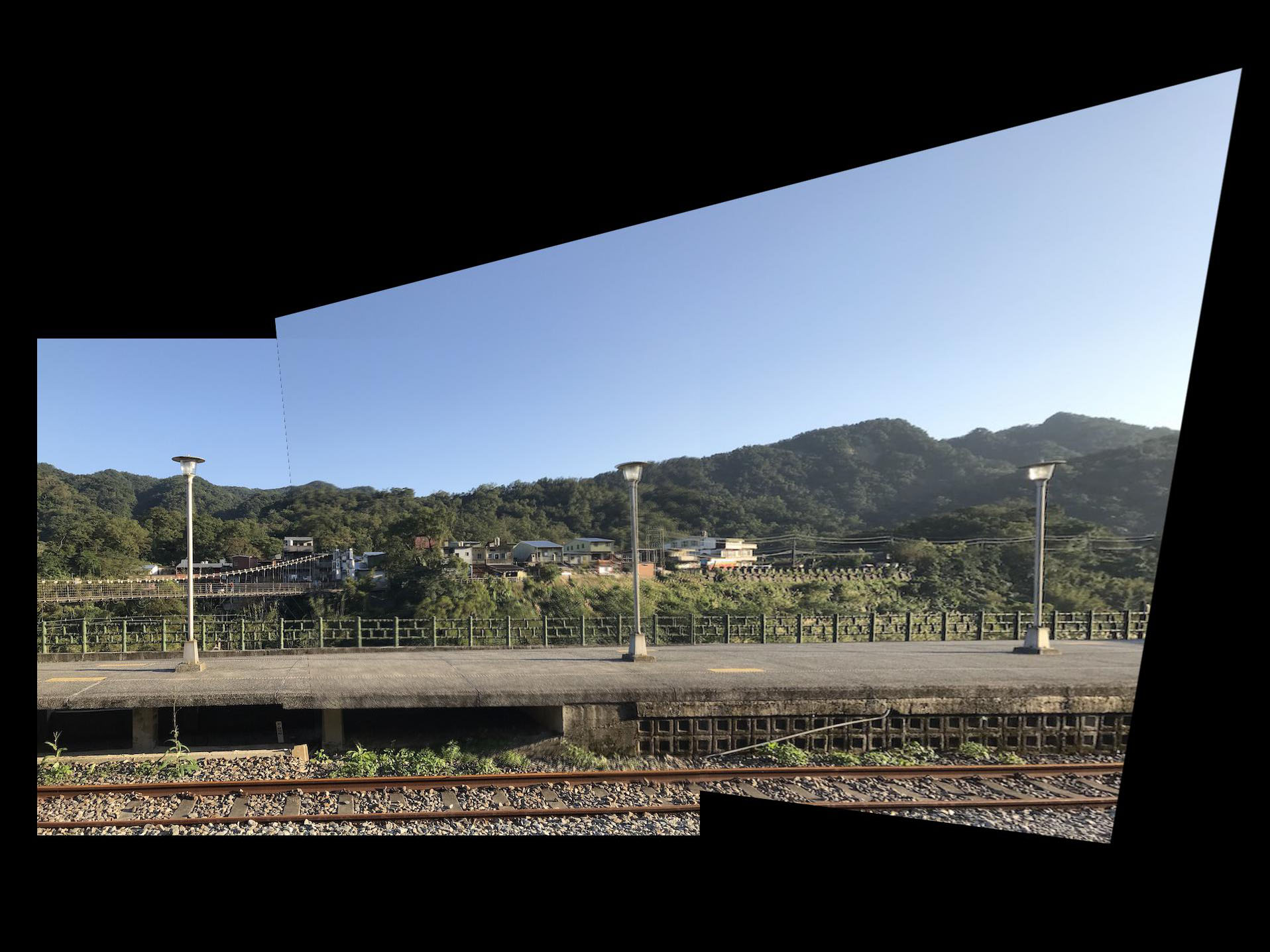
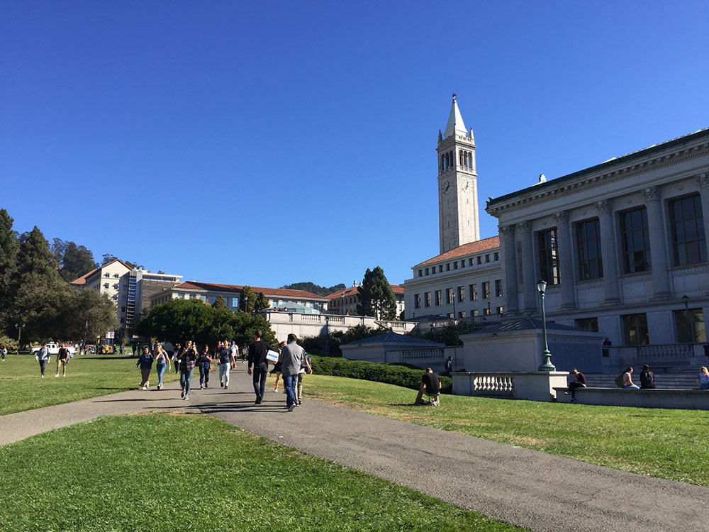
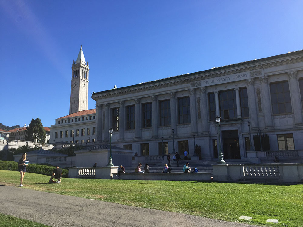
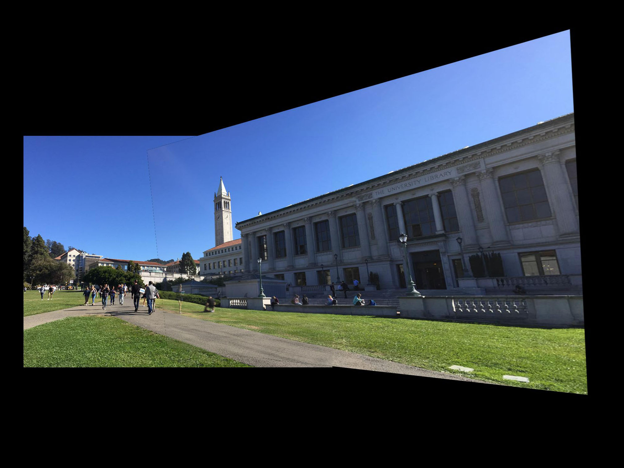
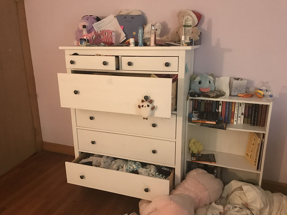
We will create a mosaic by stitching together two images that have different viewing angles from the same point of view. By using the homography matrix, we can warp one of the images to match the other appropriately. We didn't do anything special for blending, so there's a pretty obvious seam. The last mosaic didn't turn out as well as some of the others-- it's probably because it was taken with my phone camera.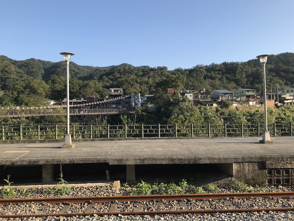
What I learned
So far, it's very cool that we can essentially warp images. It's pretty amazing how simple it is underneath the hood and that it's so simple to rectify images.Part 2: Feature Matching for Autostitching
Detecting Corner Features
We used the provided starter code to generate many potential points of interest in the images. The Harris Corner algorithm tries to find corners in an image, or points whose local neighborhoods stand in two different edge directions. Below is an example of the Harris corners found in the train image.

Adaptive Non-Maximal Suppression
Next, we implement Adaptive Non-Maximal Suppression to lower the amount of potential interest points, while also maintaining an even distribution over the image. For each potential point, we find the suppression radius: the minimum distance to nearest point that has Harris response at least 1/c * HarrisResponse(current point). We found that a c of 0.9 worked quite well, and kept 500 interest points with the highest suppression radius.
Feature Descriptor Extraction
Our next step is extracting feature descriptors from our interest points. We first take a 40x40 patch around each point and downsample it to 8x8. This helps make our features more robust.
Feature Matching
Now we try to match the features between our two images. For each feature, we find the squared distance between each feature in both images. Then, we apply the Lowe ratio test, only considering the features to match if the ratio of the distance to the 1-NN over the distance to the 2-NN is less than some threshold. We used 0.3.
RANSAC
Finally, we use RANSAC to eliminate any potential outliers. We choose 4 potential matches at random and determined the inliers and outliers. After sampling a repeated amount of times, we kept the largest set of inliers as our set of feature matches.
Mosaics
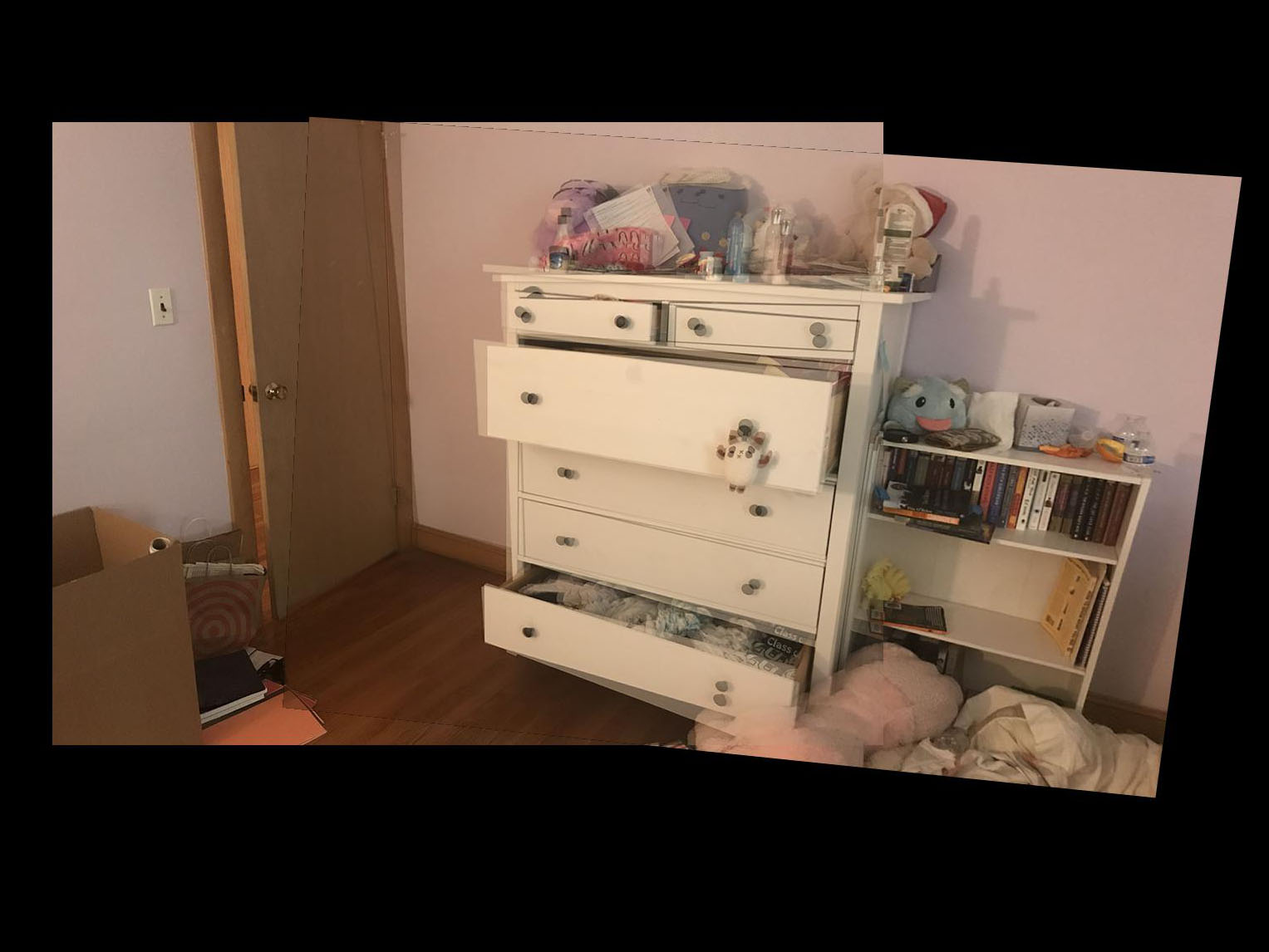
Below is a comparison between the more manually involved mosaic (left) and the automatic feature matching mosaic (right).
What I learned
I learned that the computer can do a remarkably good job automatically detecting features and matching them. It was very surprising to find out that this was not as complex as I first imagined it to be.