Image Warping and Mosaicing

Jingwei Kang, cs194-26-abr

Overview

Part 1: Image Warping and Mosaicing

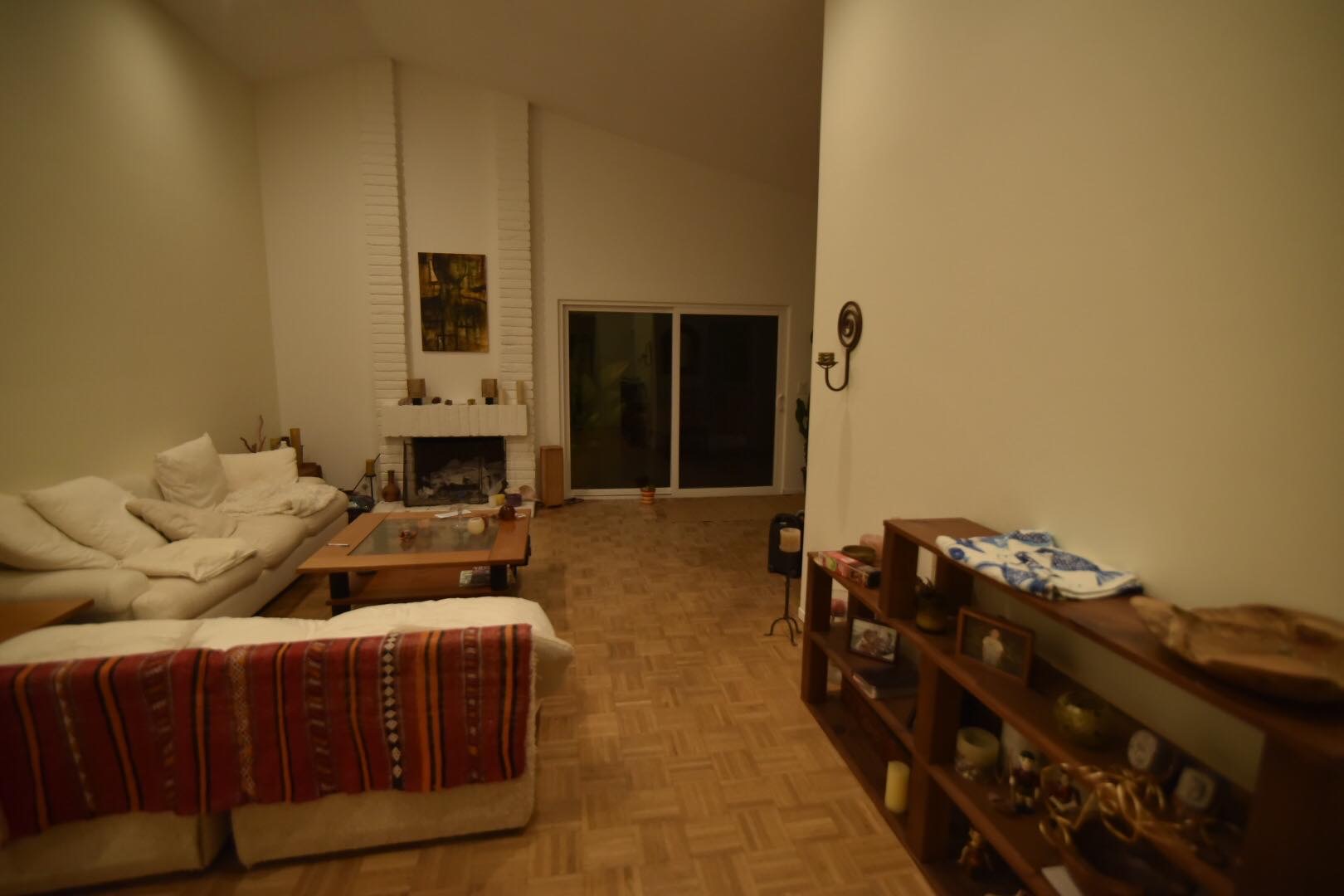
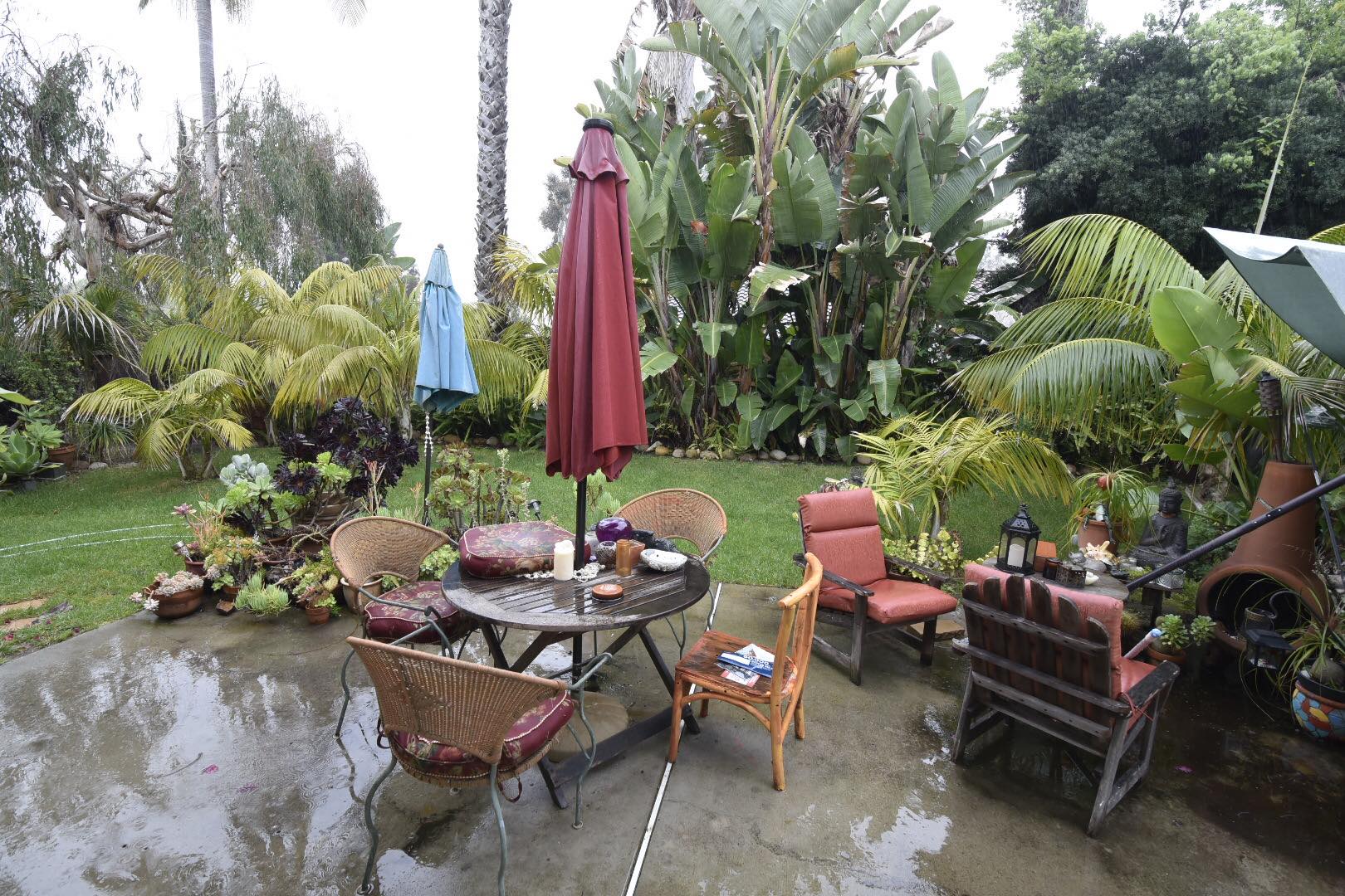
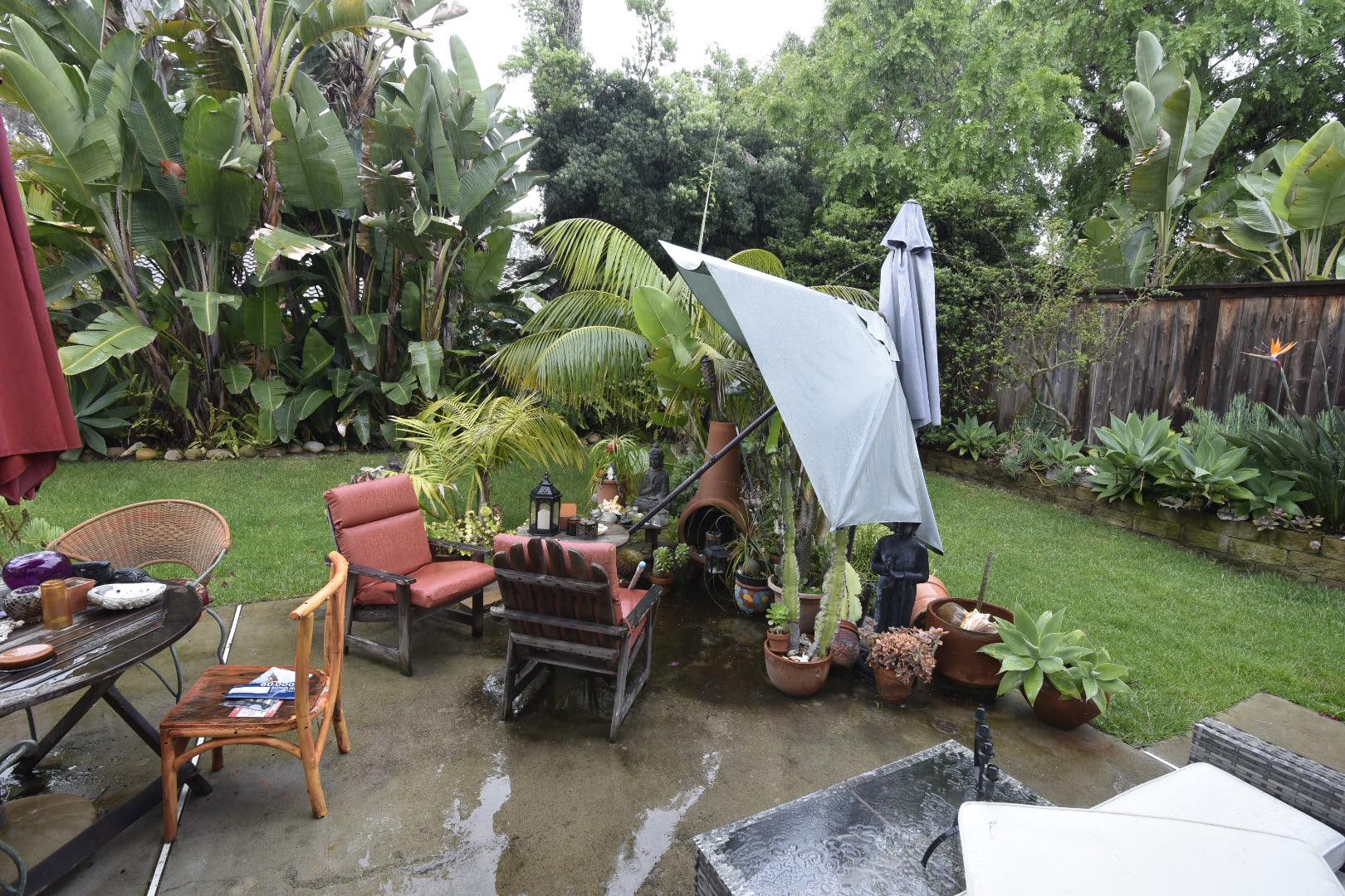
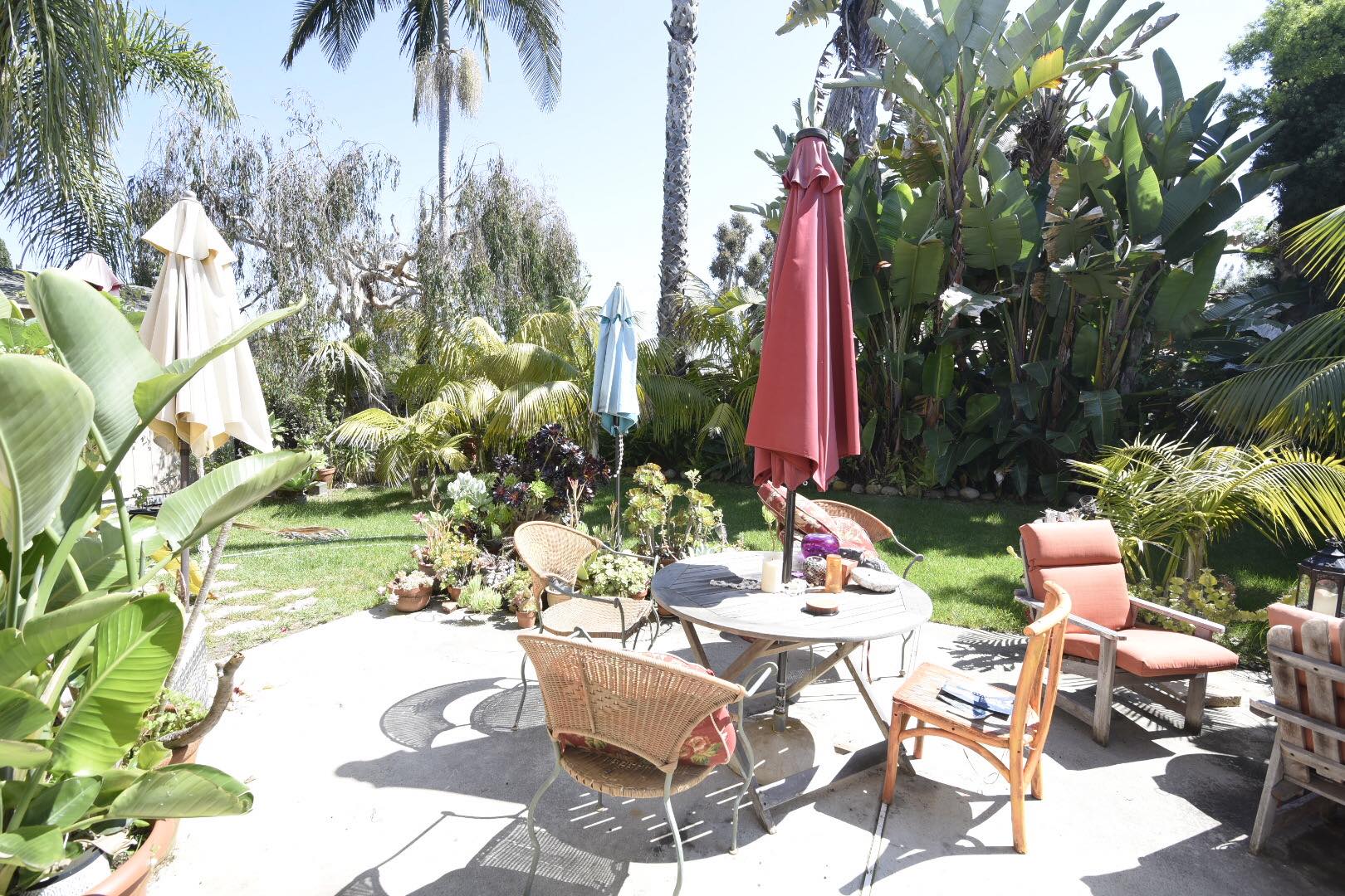
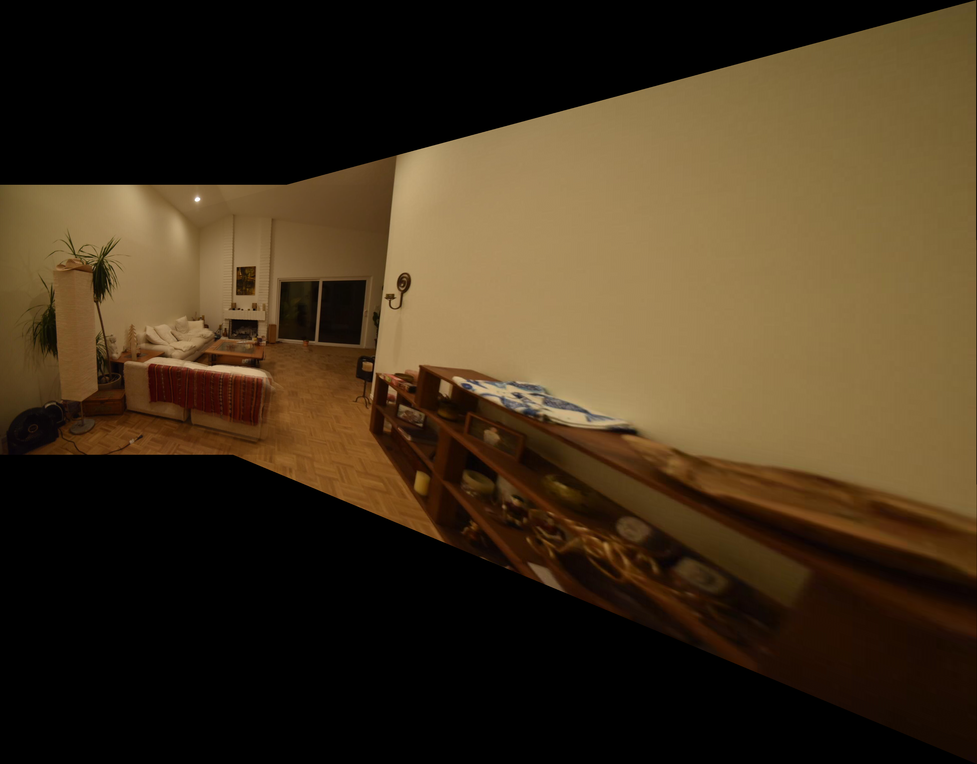
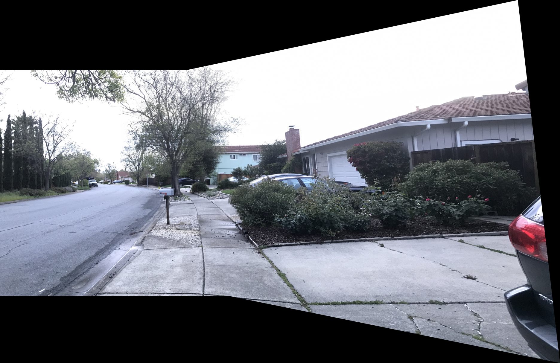
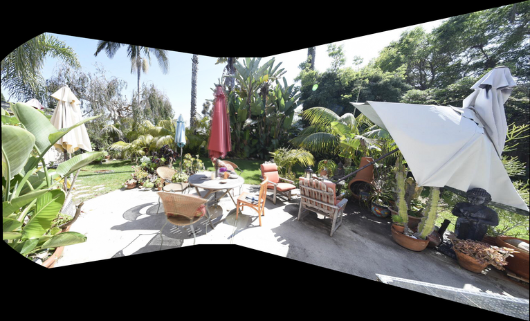
Part 1.1: Shooting and Digitize Pictures

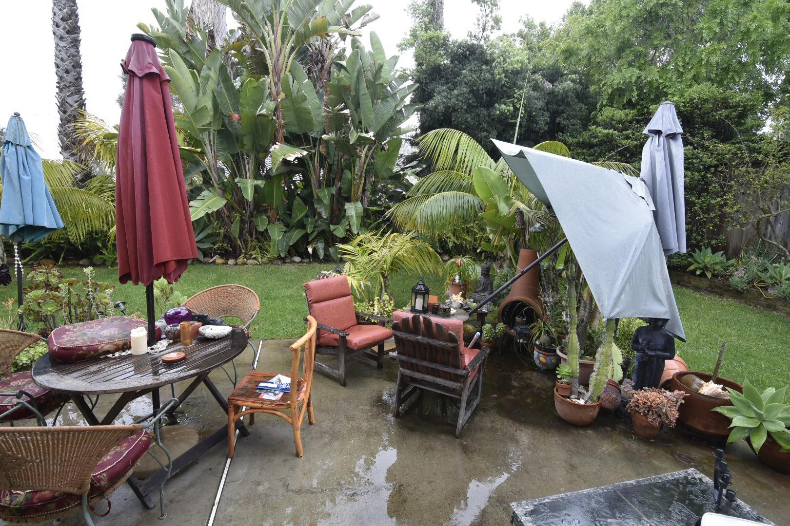
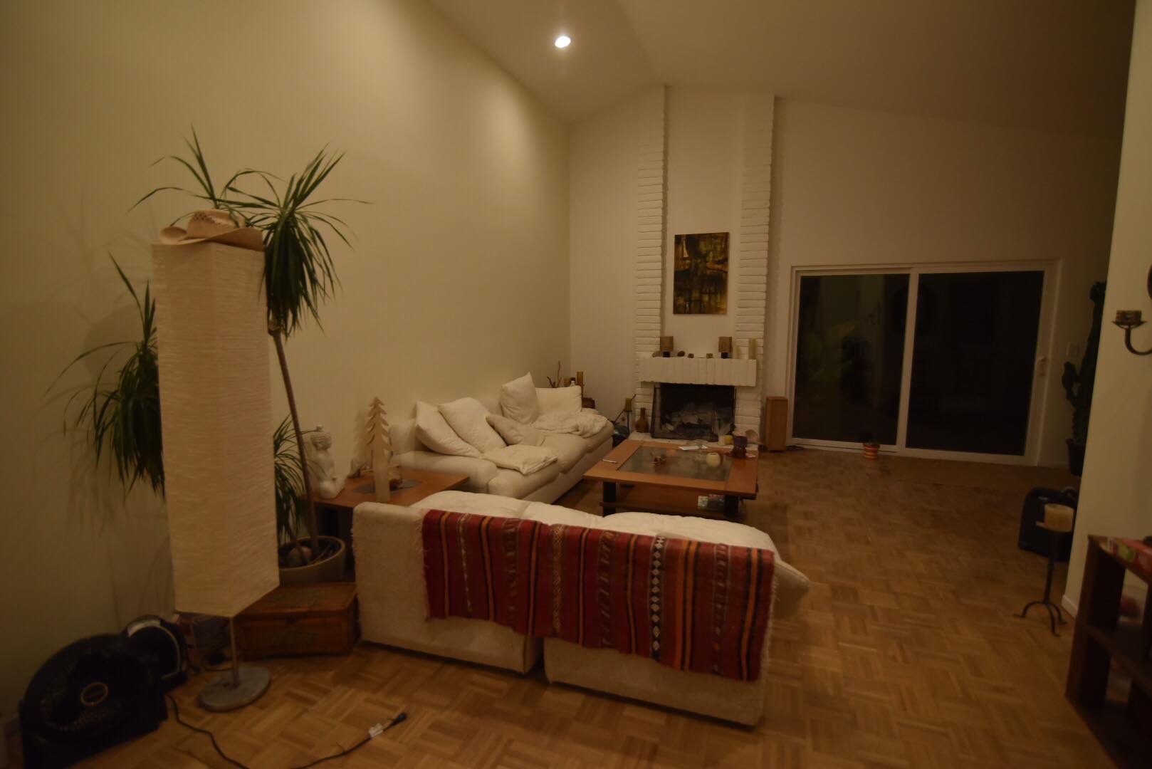
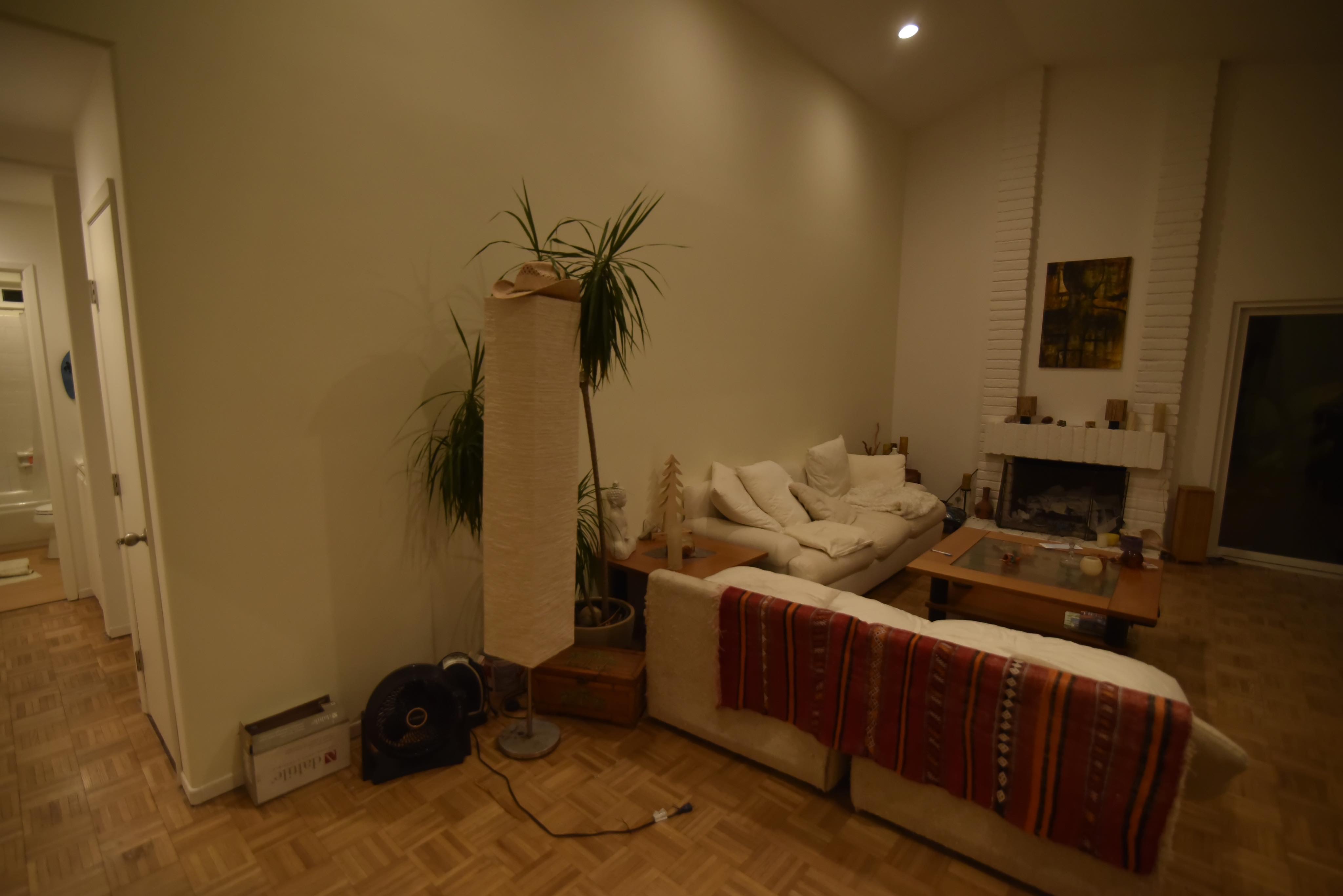
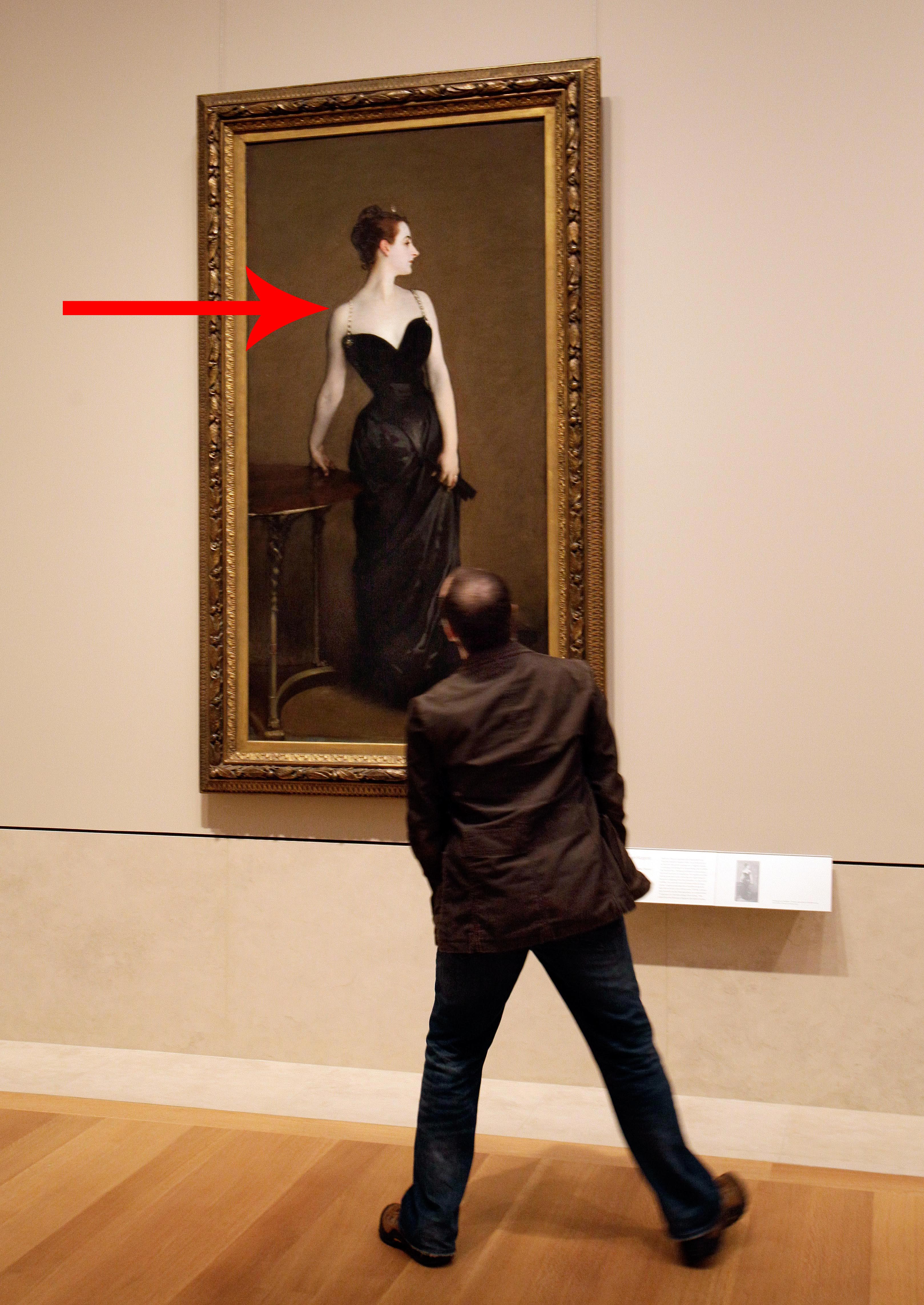
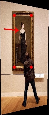
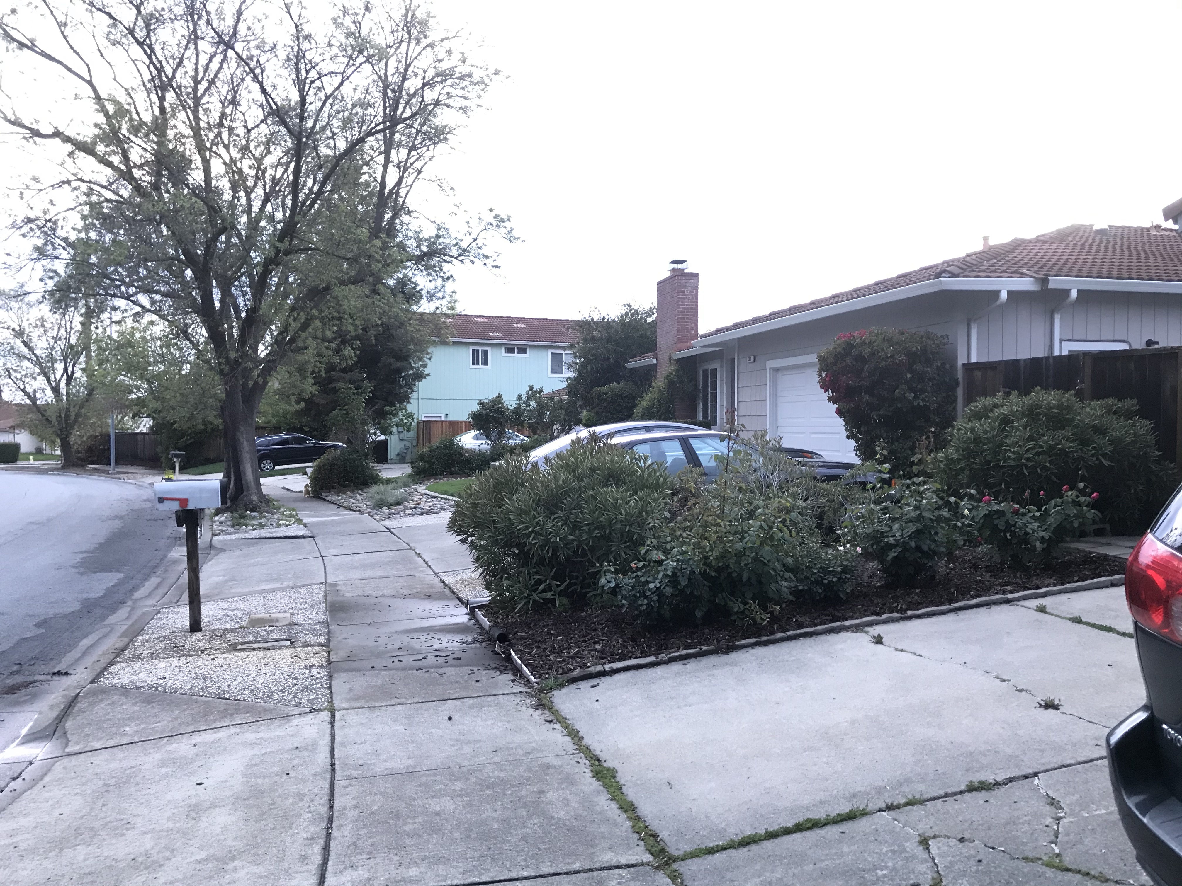
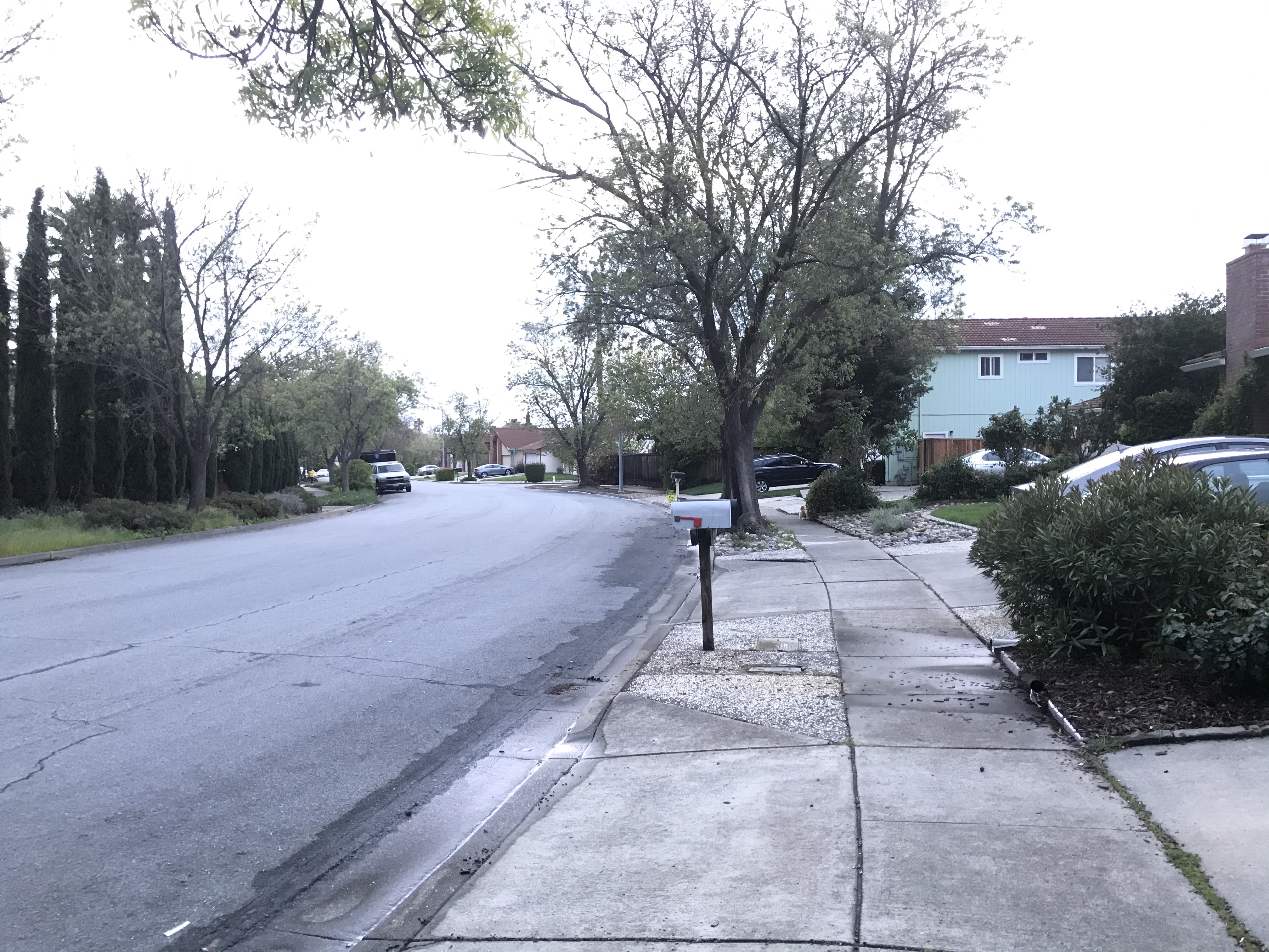
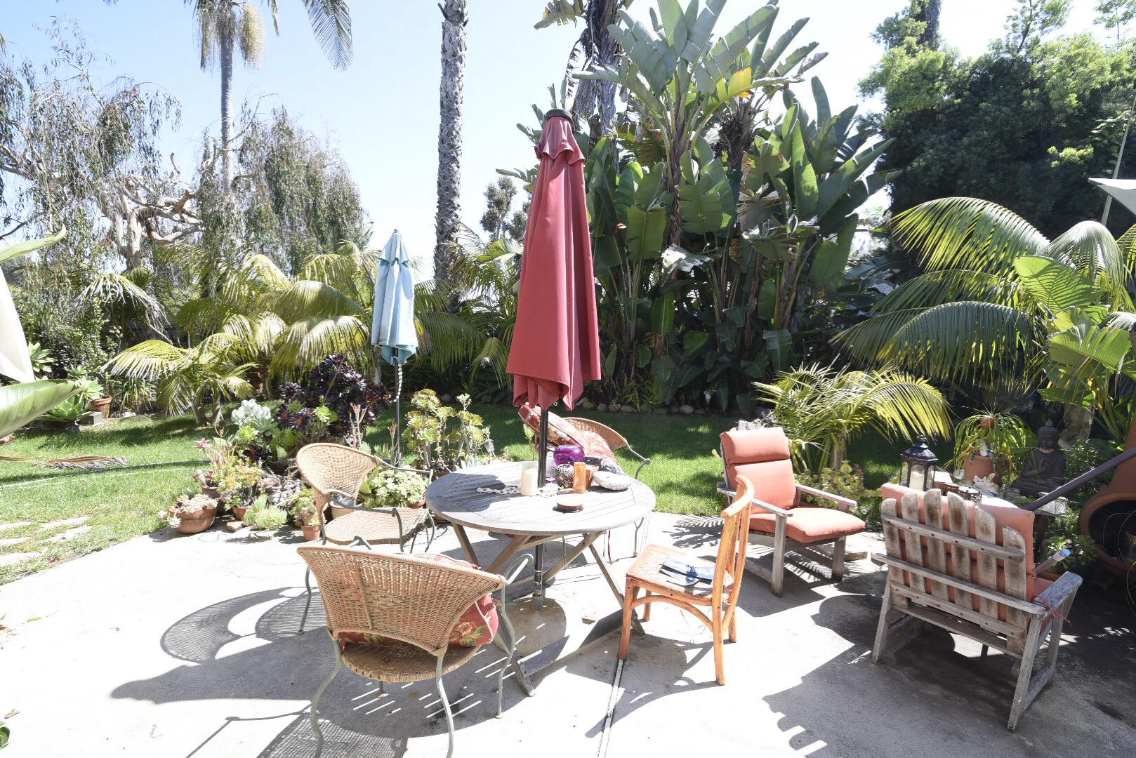
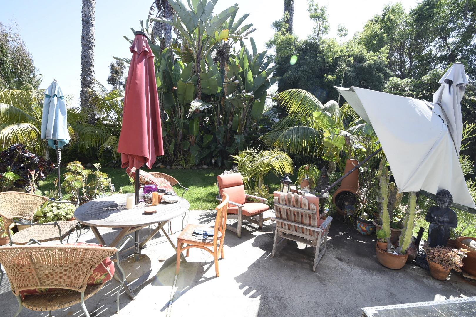
Below I've displayed a couple images I've taken of the interior and backyard of a house. I also found an image of a man observing a painting from the web that I will rectify later.

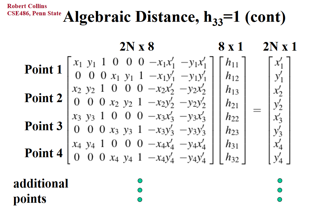
Part 1.2: Recover Homographies

Since our goal later on is to adjust our images for perspective, we need to determine the homography matrix. This matrix is 3 x 3, which is larger than the affine transformation used in project 3. As a result, we must specify more than just 3 points. In fact, we need at least 4 points, because the homography matrix has 8 free variables (each point contains and x and a y, for a total of 8 equations). To make the homography more stable, we can utilize more points and derive the least squares equation to solve the overdetermined system. I've included the final homography matrix, with the image from StackOverflow.

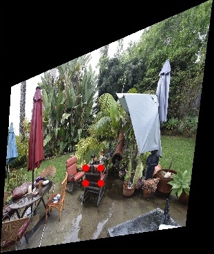
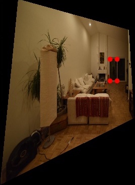
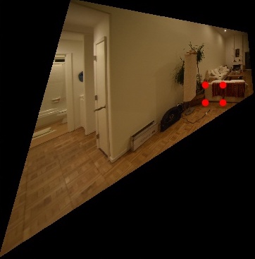
Part 1.3: Image Rectification

The procedure here was similar to that of project 3. This time, we had to account for the fact that the final image may have different dimensions after the homography mapping, but used the same inverse warping techniques. I've included some images that I've attempted to rectify (with the red points illustrating the points I selected). The image resolution may be lower here as I simply wanted to check that my homography worked without spending too much computation time.

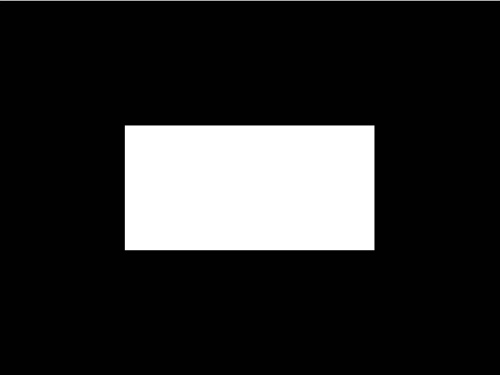
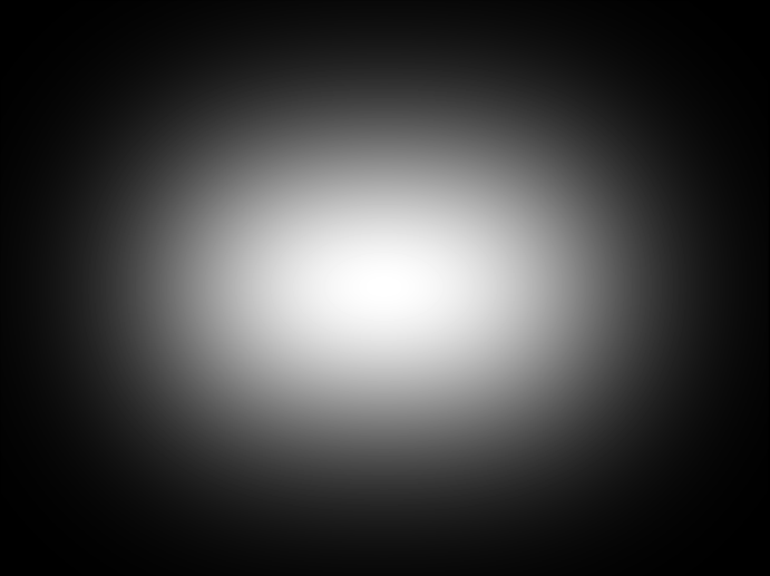
Part 1.4: Mosaics

Given that we can rectify an image with respect to a set of coordinates, we should be able to warp one image with respect to corresponding points of an image taken from a rotated viewing angle. Then, we can blend them together. To blend the warps, I created alpha channels for the images (prior to warping), which I initialized to a rectangle of 1s padded by 0s. I then applied a Gaussian filter to make this a smoother transition. These channels were then used to create a weighted average - essentially the idea is that information at the edges of an image should be weighted less to improve blending. Below are the sample filters.

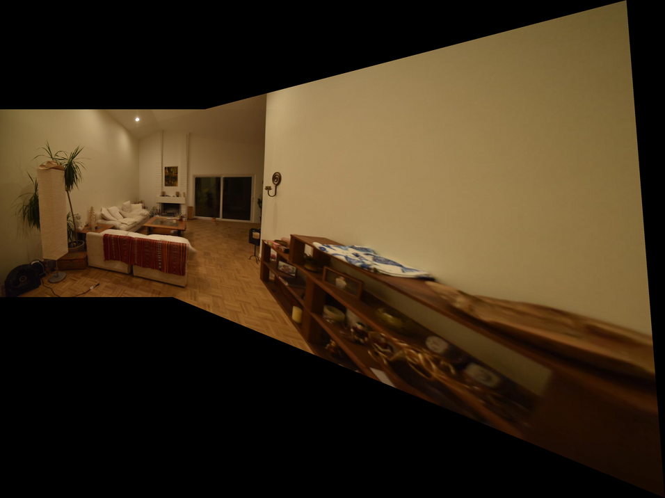
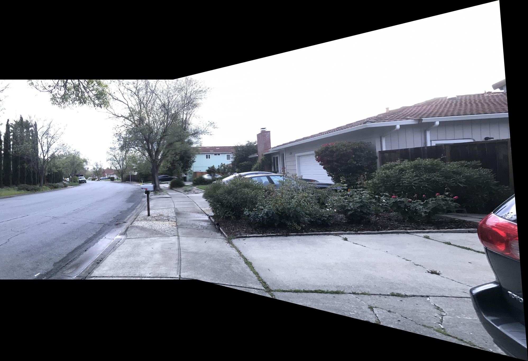
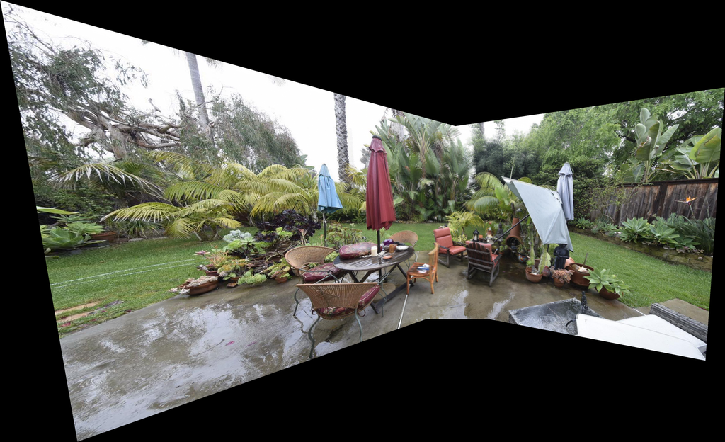
Below are some mosaics created from two images.

With this idea, we can then gradually layer on additional images to create mosaics with more images. Below is a mosaic made from 3 images.

In general, this technique works. However, we do see that the center of the image where there was significant overlap/blending appears blurry. This could be due to the fact that the images were taken without a tripod and that the projective center changed. Below I try again with a tripod.

While there does appear to be slightly less blurring when working with images taken with a tripod, this issue still persists. This is likely due to the lack of precision in my manual point selection and alignment. This problem might also be compounded by the fact that my images are taken of relatively close objects (compared to a skyline, mountains, etc.) Thus, small changes in the center of projection are not negligible and may result in some blurring. We'll see if we can improve upon the point selection and alignment when we explore automated techniques.

Part 2: Feature Matching for Autostitching

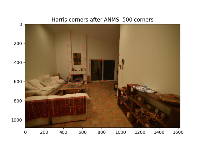
Part 2.1: Detecting Harris Corners

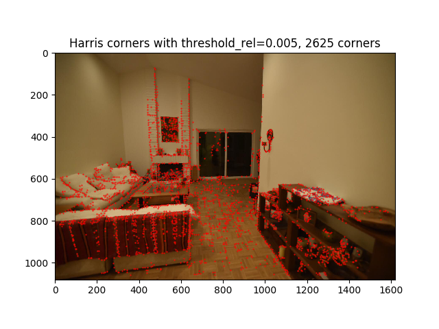
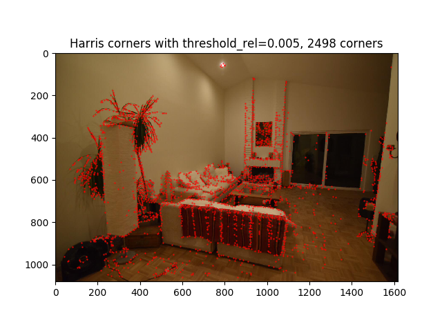
First, we want to extract features in our images that we can use to determine homographise and warp images for stitching together. One common feature is the Harris corner, which we detect using the code provided in the project (which uses functions in skimage.feature). The original code generated upwards of 35,000 Harris Corners for each image. To reduce runtime in later steps, I increased the threshold and the minimum distance between corners used in the skimage functions.

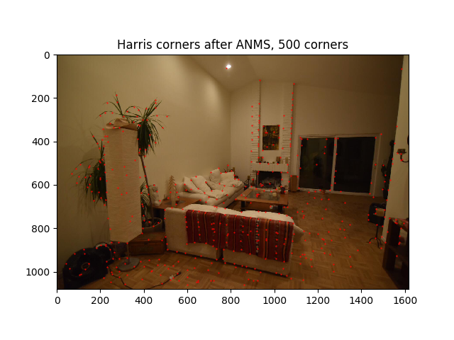
Part 2.2: Adaptive Non-Maximal Suppression (ANMS)

While adjusting the threshold greatly reduced the number of Harris corners, we still have far too many. Furthermore, we don't want to have clusters of corners - imagine having a small overlap between images but all corners are clustered outside of the overlap. In that case, finding the homography would not be possible. To ensure a more even distribution, we use Adaptive Non-Maximal Suppression from the paper with a constant of robustness of 0.9. Essentially for each corner, we find a minimum distance/radius to a corner that is reasonably larger than it (in terms of Harris response matrix). Then, we order the radii in decreasing order and select the 500 corners with the largest radii. This ensures a more even spread as seen below.

Part 2.3: Feature Extraction

From each corner, we extract a feature - essentially a 40 x 40 patch that we blur down to 8 x 8. We also make sure to normalize the pixel intensities to a mean of 0 and standard deviation of 1. These steps are important to making the features invariant to changes in intensity and scaling.

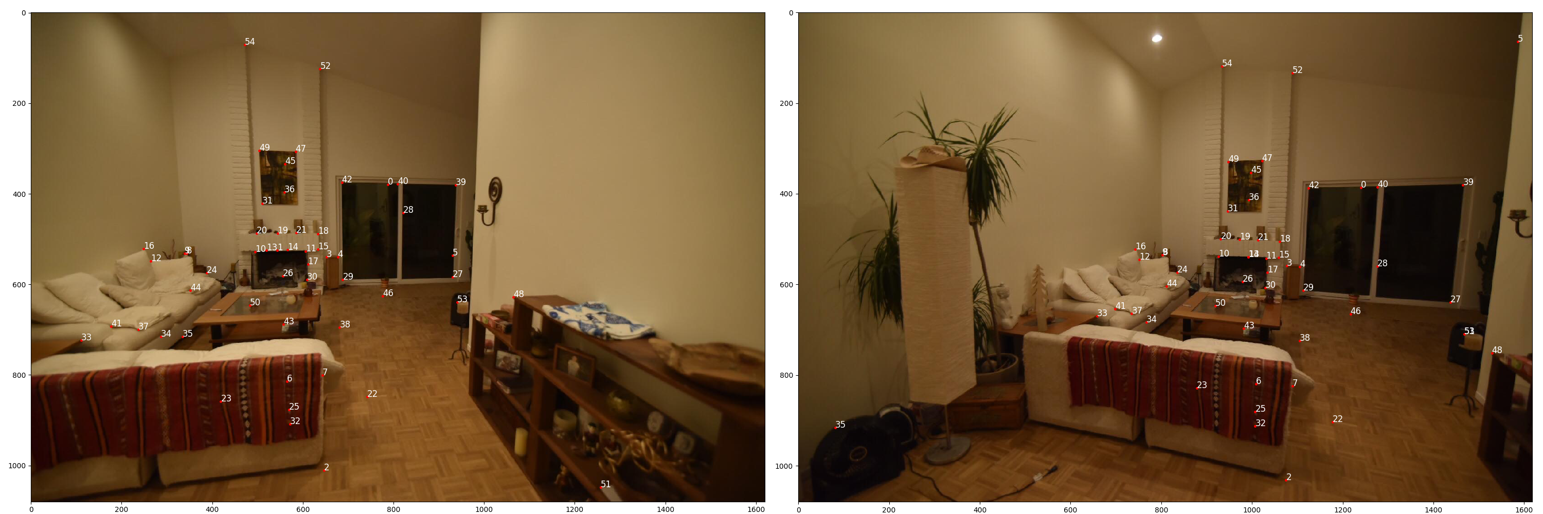
Part 2.4: Feature Matching

Next, we want to match corners between the two images. We start by computing the SSD (Sum of Squared Differences) between pairs of features (in opposing images). Following Lowe's outlier rejection, we compute a ratio for each feature which compares the SSD of the closest match and the second-closest match. Intuitively, if a match is correct, it should be significantly better than all other possible matches. Using Figure 6b in the paper, I selected a threshold of around 0.5, which seems to be where we can capture a good number of correct matches without seeing too many incorrect matches. Although the text in the figures are small, we can see upon closer inspection that our features (points) are matched pretty well.

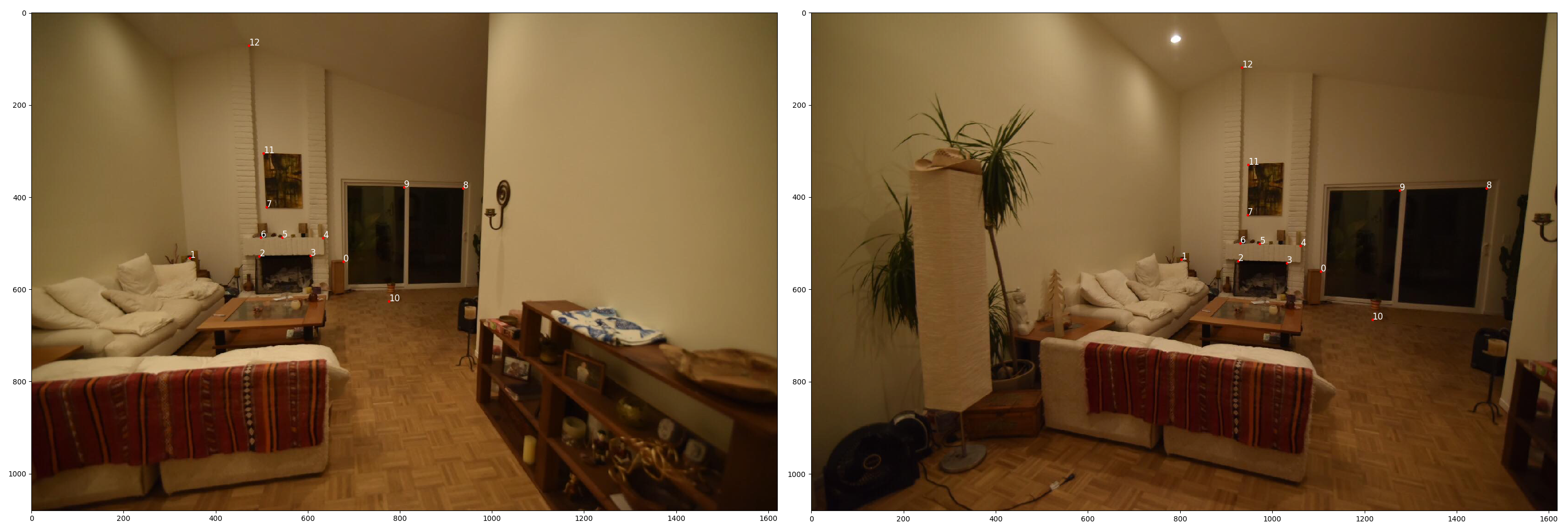
Part 2.5: Random Sample Consensus (RANSAC)

Regardless of how we threshold, it's still possible that we have incorrect matches. We know that incorrect matches can significantly reduce the accuracy of our homographies, so we use the RANSAC algorithm to further screen out bad matches. Essentially, we randomly select 4 feature matches at a time and use them to compute a homography. We then use this homography to transform all the features (coordinates) from one image, and see how close they land to the corresponding feature (coordinate) in the second image. Those that have an SSD within a certain tolerance (I used 0.3) are called "inliers". We run this loop multiple times (I used 2000 iterations) and keep the largest set of inliers. Note how in the previous image, point 35 (on the fan in the lower left corner of the right image) is clearly matched incorrectly. In the image below, the numbering isn't identical but we can see that we only retain the correct matches.

Part 2.6: Autostitching

Once we've computed the largest set of inliers, we can use them to compute a robust homography estimate as we did in part 1 and mosaic the images together. We can also create mosaics from more than 2 images by chaining together the operations as in part 1.

As we can see, the results are pretty similar, without the painstaking point selection! Note that in the room example, the homography calculated was different because different points were selected. We can see from Part 2.5 that the algorithm selected points further in the distance, whereas when I manually aligned them I selected points on the the backs of the couches as well. As a result, we can see that the autostiched image has more blur near the couches but less into the distance. It doesn't seem like it was possible to align these images perfectly, which is to be expected given that they make up a "close-up" panorama, and changes in the center of projection are more noticeable.

Takeaways

There was so much to learn from this project and it was extremely rewarding after realizing how tedious manual point selection is. An interesting concept I learned in this project was that that garbage in = garbage out. It's not possible to generate new data from projecting and existing image (i.e. if we can't see something hidden behind a couch in one image, that's going to be the case regardless of how we project). Thus, this makes it critical to keep the same center of projection for this panorama stitching application.