Part 1: Image Warping and Mosaicing
Objective
We use our knowledge of projective transformations and homographies in order to stich a mosaic from two pictures taken at the same location but different perspectives.
Recover Homographies
Finding the \(H\) homography matrix is a similar process to the image morphing from project 3. Whereas the affine transformation in project 3 uses 6 degrees of freedom, the projective transformations for perspective shifts require 8. Mathematically, it takes the form \(p' = Hp\) where \(p\) is the original point and \(p'\) is the projected (transformed) point.
\[\begin{bmatrix} wx' \\ wy' \\ w \end{bmatrix} = \begin{bmatrix} a & b & c \\ d & e & f \\ g & h & 1 \end{bmatrix} \begin{bmatrix} x \\ y \\ 1 \end{bmatrix}\]
It turns out that \(w\) is a scaling factor that should be divided out to get the correct final location location. To find \(H\) numerically, we rewrite the matrix multiplication in the following form:
\[\begin{bmatrix} x_1 & y_1 & 1 & 0 & 0 & 0 & -x_1x_1' & -y_1x_1' \\ 0 & 0 & 0 & x_1 & y_1 & 1 & -x_1y_1' & -y_1y_1' \\ x_2 & y_2 & 1 & 0 & 0 & 0 & -x_2x_2' & -y_2x_2' \\ 0 & 0 & 0 & x_2 & y_2 & 1 & -x_2y_2' & -y_2y_2' \\ \vdots & \vdots & \vdots & \vdots & \vdots & \vdots & \vdots & \vdots \\ x_n & y_n& 1 & 0 & 0 & 0 & -x_nx_n' & -y_nx_n' \\ 0 & 0 & 0 & x_n & y_n & 1 & -x_ny_n' & -y_ny_n' \end{bmatrix} \begin{bmatrix} a \\ b \\ c \\ d \\ e \\ f \\ g \end{bmatrix} = \begin{bmatrix} x_1' \\ y_1' \\ x_2' \\ y_2' \\ \vdots \\ x_n' \\ y_n' \end{bmatrix}\]
With 8 degrees of freedom and each point correspondence providing 2 degrees of information, we need at least 4 point pairs to uniquely define a homography matrix. However, labeling additional points and using the least-squares formula (since it takes the form \(Ax = b\)) to reduce reconstruction error makes our projection more robust to noise. Once the column matrix is calculated, we simply append the final 1 at the end and reshape it to form our 3x3 \(H\) matrix.
Image Rectification
Once the homography matrix is found, we need to warp the original image into the new shape. Unlike the morphing project, where the warped image is guaranteed to still lie in a valid region, it is possible that some regions from the projective transformation lie out of bounds. This leads to additional complications and telltale black regions in the warped images.
For the warping itself, I used an inverse-warping procedure with nearest neighbor interpolation. I did not see major aliasing artifacts to justify using more complex interpolation procedures, especially considering the size of the original images I chose.
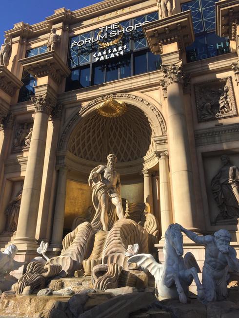
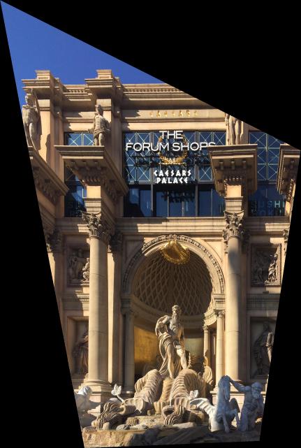
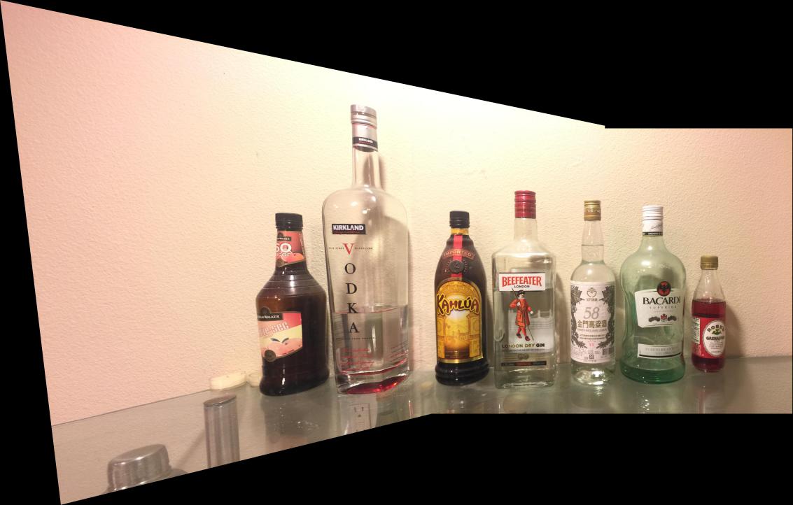
As a sanity check, I found a photo from my last Las Vegas trip of Caesar's Palace taken at an off-center perspective. I used homographies to try to better realign the image to what it would look like when viewed dead on. Even though I only used the minimum four correspondence points, the result looks surprisingly realistic.
Continuing the theme of misaligned Vegas resorts, here is a rectified version of the Bellagio. While rectification can mimic a perspective shift, it cannot add new optical information from another vantage point. We can still see the left side of the hotel, which should not be possible when viewed dead on.
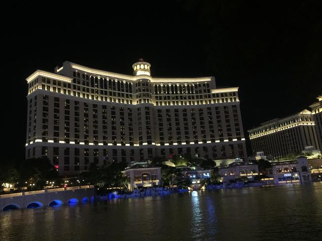
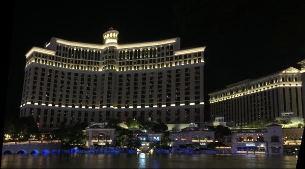
Image Mosaic
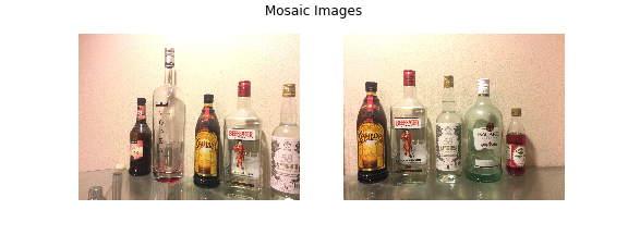
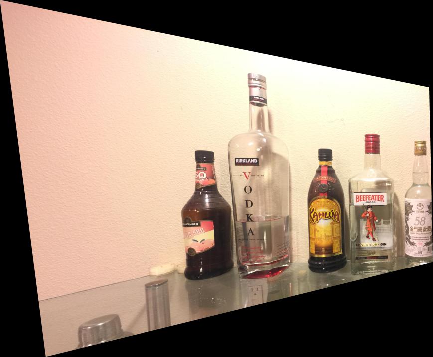
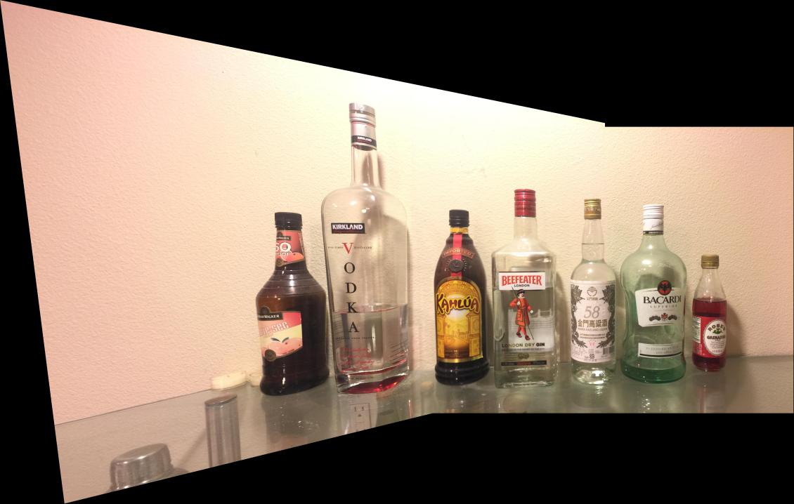
We can now put everything together to form the image mosaic. I found seven correspondence points between the two images of bottles of wine, and calculated the homography matrix required to warp one image to the other. I had to handle the different offsets from warping to ensure that the two images were still properly aligned. Below, I included the picture of the warped first image as well as the finished mosaic. I used the assumption that the brightness of the two images were about equal, and simply divided the overlapping region by 2. Despite being a simple hack, it worked wonders in removing edge artifacts.
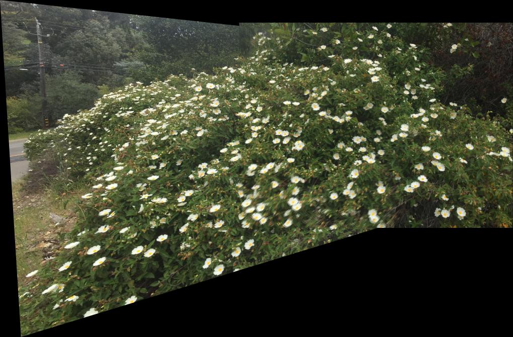
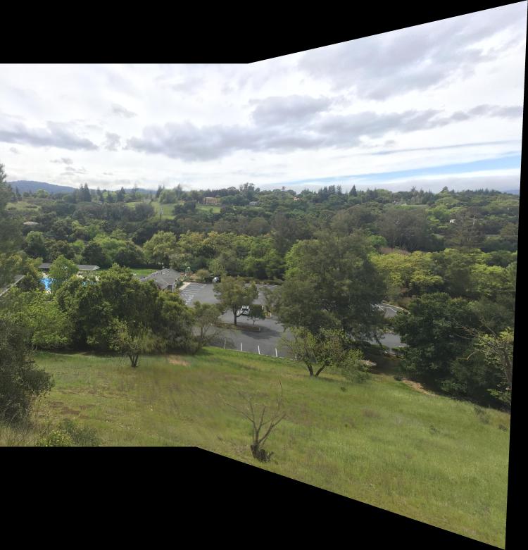
I repeated the same process to compute a mosaic for a flower bush and a country club. For the country club, I switched up the blending to have the right image warped into the left one. I also slightly cropped it for viewing convenience.
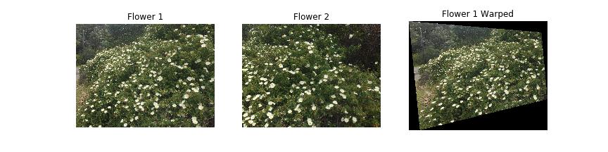
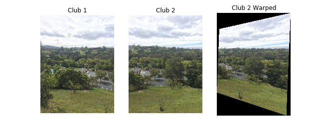
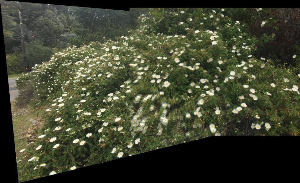
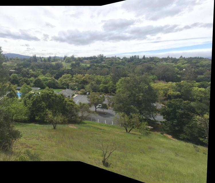
While the country club mosaic looks seamless, the flower bush is blended poorly in the bottom middle region. Ironically, that image had the most correspondence points. In retrospect, choosing a flower bush with few outstanding features makes manual labeling difficult and error-prone.
Takeaways
This part feels like a step up from the image morphing of project 3. Projective transformations do add a layer of difficulty. I had a failure case where I made my transformation too sharp (angle-wise, though I also did use full-scale resolution), resulting in a memory shortage error. In that scenario, warping both images into a middle perspective rather than from one image to another would be ideal; however, I had no intuition for how to manually label those correspondences.
I learned that panorma images are highly sensitive to photo shooting techniques. In addition to the angle dilemma above, keeping the camera position constant and ensuring even brightness pay dividends later in the processing stage. I was lucky to not hit many issues that require more complex techniques and algorithms.
Part 2: Feature Matching and Autostitching
Objective
We use feature extraction and matching to automatically align our images for better quality and convenience. I used the autostitching procedure outlined in the linked paper on the same images as part 1 so that comparisons can be made.
Corner Detection
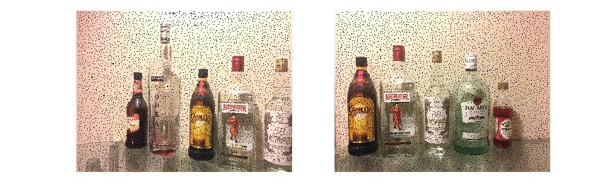
I integrated the given Harris detection code into the project. Given that I used full-sized images, I adjusted the minimum distance to 20 pixels apart to keep my corner count lower. For reference, after adjusting minimum distance, the number of corners in my picture were in the order of thousands.
Adaptive Non-Maximal Suppression
Thousands of corners is a lot for even computers to process. I implemented ANMS as described in the paper to reduce the number of corners to a managageable size. The algorithm weights a Harris corner \(x_i\) by its distance to the closest Harris corner \(x_j\) of moderately greater weight. The paper used a robustness constant \(c_r\) of 0.9, meaning that the neighboring corner must be 11% stronger to be considered.
\[ r_i = \min_j |x_i - x_j|, ~\text{s.t.} f(x_i) < c_r f(x_j) \]
Smaller distances mean that there is a stronger corner nearby, whereas larger distances imply that there are no better corners in the vicinity. The algorithm orders the corners from largest radius to smallest radius and takes the first \(N\) points. ANMS is better than naively taking the \(N\) strongest points because it takes the spread of corners aorund the image into account. The naive method may choose corners from only a small portion of the image, which will eventually fail to match corners if the actual overlapping section is far.
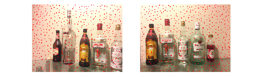
I implemented ANMS and took the 500 largest corners, a default given in the paper.
Feature Extraction
We extract a feature descriptor from each corner to prepare for the matching process. This entails getting a 40x40 pixel square around the corner and downscaling it to an 8x8 patch for robustness sake. This is demeaned and normalized to make comparisons across descriptors easier.
Feature Matching
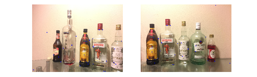
We now use the feature descriptors to try to find matching corners between both images. We use brute-froce to find the distances between the 500 features in one image to each of the 500 corner features in the second. For each corner, we then evaluate the two corners in the opposite image with the smallest distances. The theory is that if two corners are truly corresponding, there should not be a third corner of similar distance. Two corners are considered "corresponding" if the ratio of the distance to the first nearest neighbor and to the second is under a certain threshold. There is a balance between having too few matches and too many false-positives. I chose a threshold of 0.5 and out of the 500 potential pairs, I ended with 30 corresponding points (in blue).
RANSAC
To robustly compute a homography despite false positives in matching, we use the RANSAC algorithm. It randomly chooses 4 of the pairs, computes the homography matrix, and sees how many of the pairs "agree" with the transformation. The intuition is that false positives are random, but the true positives follow the transformation signal. After repeating this thousands of times, we keep the most agreed transformation. After implementing RANSAC, my 30 matching pairs got reduced to 10 pairs (in green). This implies that I could probably have used a smaller threshold in feature matching.

Warping and Blending
The rest of the procedure follows part A. We have our automatically generated correspondence points to compute the homography transformation to blend the images. Below, I included both the automatic and manual stitchings for comparison.
| Manual | Automatic |
|---|---|
|
 |
|
 |
 |
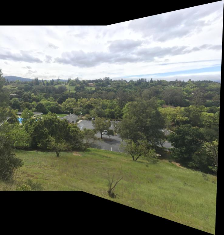 |
The results were mixed. The wine images look identical to me. The automatic process did a better job for the flower image; however, there is still minor blurriness in the bottom middle. This can probably be chalked up to the parallax effect from a slightly different angle, especially considering that the bush was directly in front of the camera. Small changes in the flower positions due to wind could also play a factor. For the country club, the manual image is slightly better in my eyes. The leafless bush in the very front is the biggest difference, with the automatic version being blurrier. I did use the bush as one of my correspondence points in manual alignment, however.
Despite its possible flaws, the autostitching produced equal caliber mosaics with far less of the painstaking work required to find, label, and type in correspondence points.
Takeaways
Professor Efros has mentioned the project topics throughout the semester, and this project is the one that I've always found the coolest conceptually. While frequency analysis and CNNs might be more relevant or cutting-edge in the modern world, there is still something inherently cool of putting two images together like a jigsaw puzzle. Having finishd the project now, I found the results rewarding to see. I am especially surprised with how well the automatic version tunred out; it ran very quickly and after writing the code, it is much easier to run than the manual stitching. Generating new mosaics is a matter of dropping two images down the toolchain.
Similar to what I mentioned in the previous part, the biggest thing I wanted to improve on is to create a final projection to warp the images towards, rather than warping an image to another sequentially. While it is possible to warp the final blend into the desired perspective, I feel that direct translations would be better. If nothing else, the reduced number of transformations would lead to less information loss.
Part 3: Large Scale Mosaic
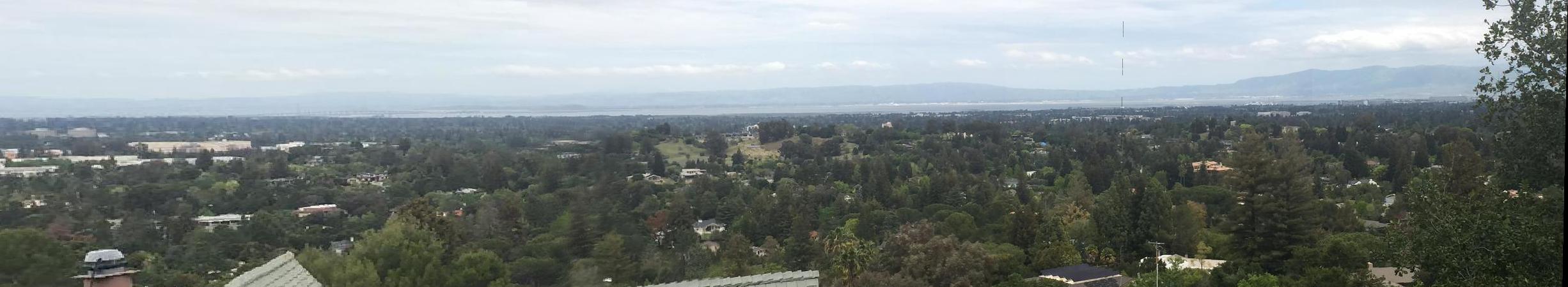
When working on the project, I personally wanted to create a large panorama using multiple images. (This is not a Bells and Whistles task). I hiked to the top of a hill overlooking the Bay Area and took four pictures to stitch together. If you look closely at the first picture, you can even see the Dumbarton bridge.
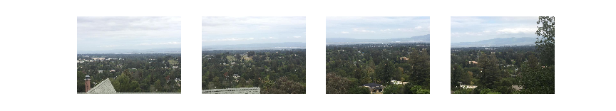
I wanted to have the computer automatically stitch the panorama together but the first three images were spaced too far apart, leaving me no choice but to manually label correspondences again. There ended up being a minor edge artifact on the right side of the image (boundary between pictures 3 and 4), though I suspect that was due to aliasing effects when I downsized the image. Funny enough, it looks like a natural antenna.
Behold my grand finale for this project, the Bay Area panorama.