Part A: Image Warping and Mosaicing
Just for the checkpoint, I implemented simple rectification of an image taken at an angle
using homography. First, I defined a function that given two sets of correspondence points, found
the homography transformation matrix that takes one to the other using least squares. I then took an
angled photograph of another picture on my wall, and selected correspondence points on that photograph
at each of its four corners. I then defined another set of correspondence points equivalent to just a simple
rectangle. From there, I found the H matrix using my function that I defined with those two
sets of correspondence points, and then for each point position in my original image, found the
inverse warping equivalent pixel from the angled image. After finding this matching, I filled in the pixels accordingly,
to create my rectified image! Below are my original, and then rectified images:
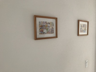 Original
|
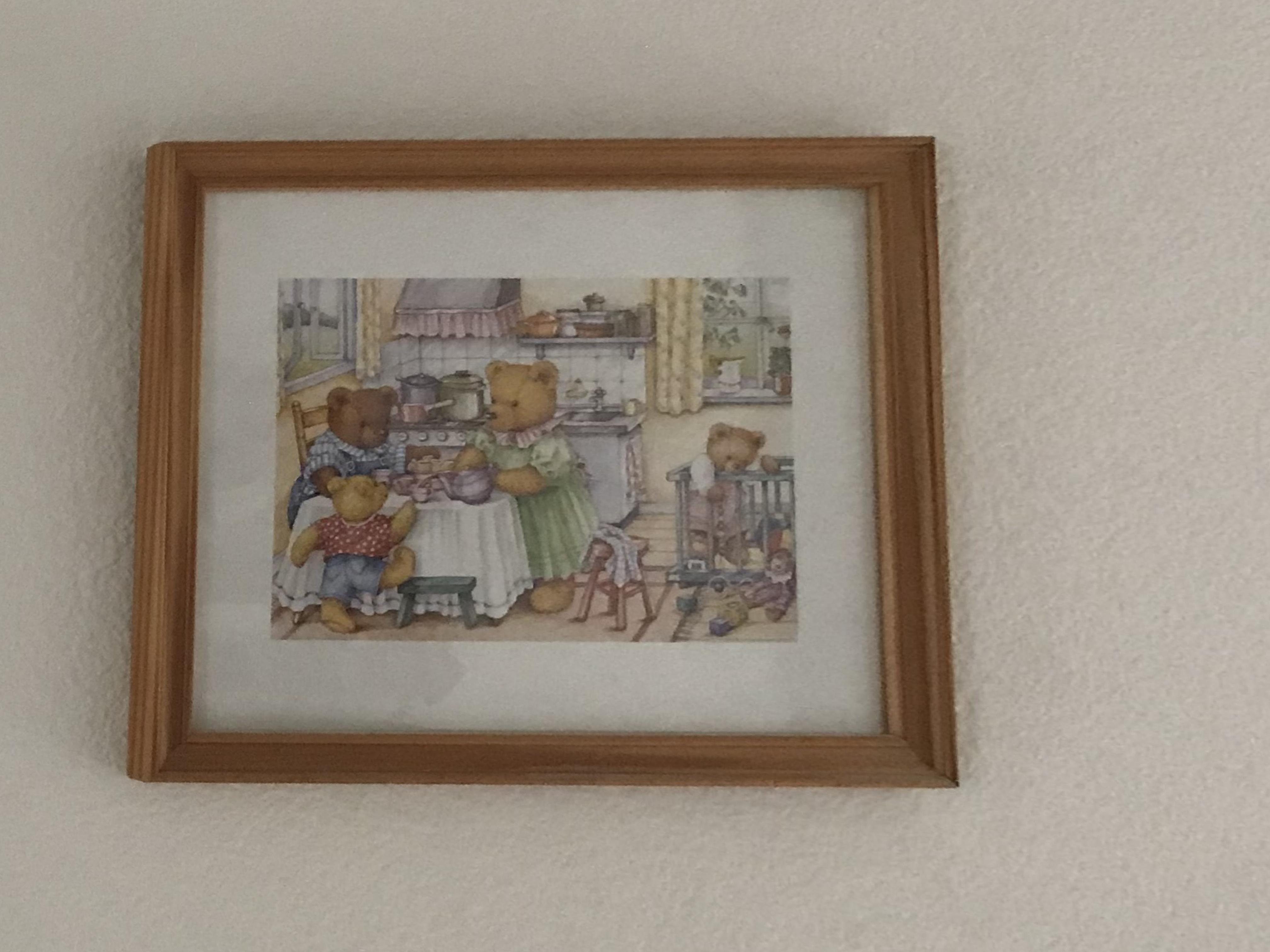 Rectified
|
Here is another example of me using rectification, this time on a light switch on my wall:
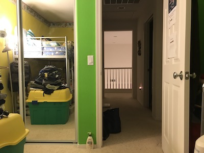 Original
|
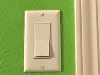 Rectified
|
Next, I took pictures of parts of my house, and manually set correspondence points in
order to align and blend them into a mosaic. I used the same technique as in Project 3,
except using a homography instead of an affine transformation, to compute the inverse warping
between two images, in order to warp one to the alignment of the other one. I managed to do
this for various pairs of pictures, manually defining the correspondence points by hand to
create the corresponding homography transformation between them. I also used alpha blending
to smooth out the edges of the pictures for alignment, multiplying pixels by constant values
between 0 and 1 that increased to 1 as they got closer to the center. This allowed for the
edges to become smoother between images, although it did create slightly darker images in
certain areas of the panorama.
Below are the source images and resulting mosaic of three different attempts at manually
defining correspondence points of images in my own house, and one from the provided source
images. I used a total of 10 - 12 correspondence points per image, which resulted in some noise
between the two, although this could be corrected depending on the precision of those points
or just including more in general:
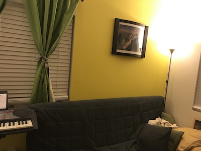
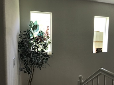 Wall: Left
|
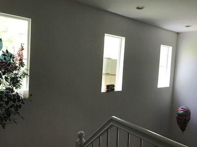 Wall: Right
|
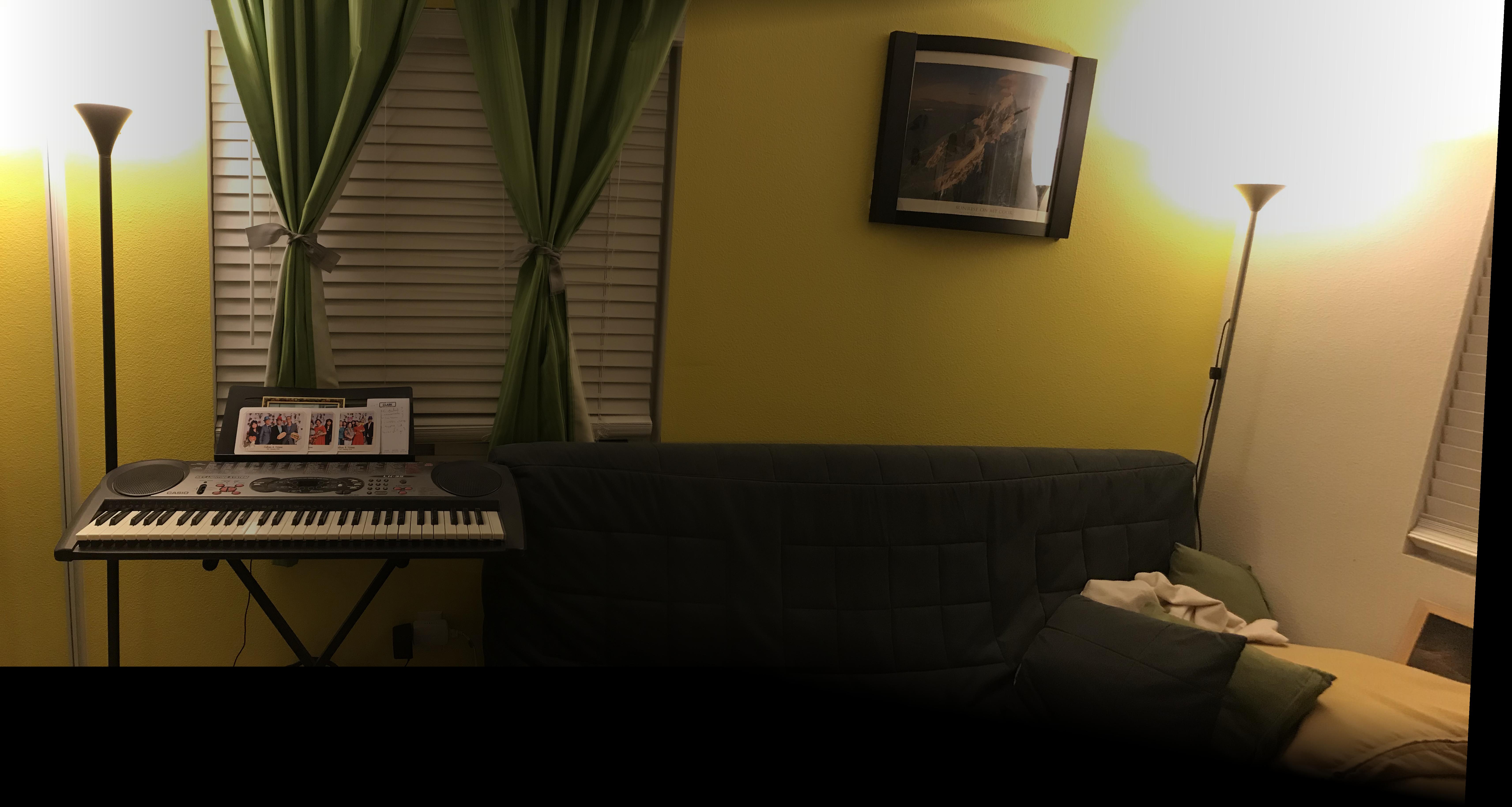
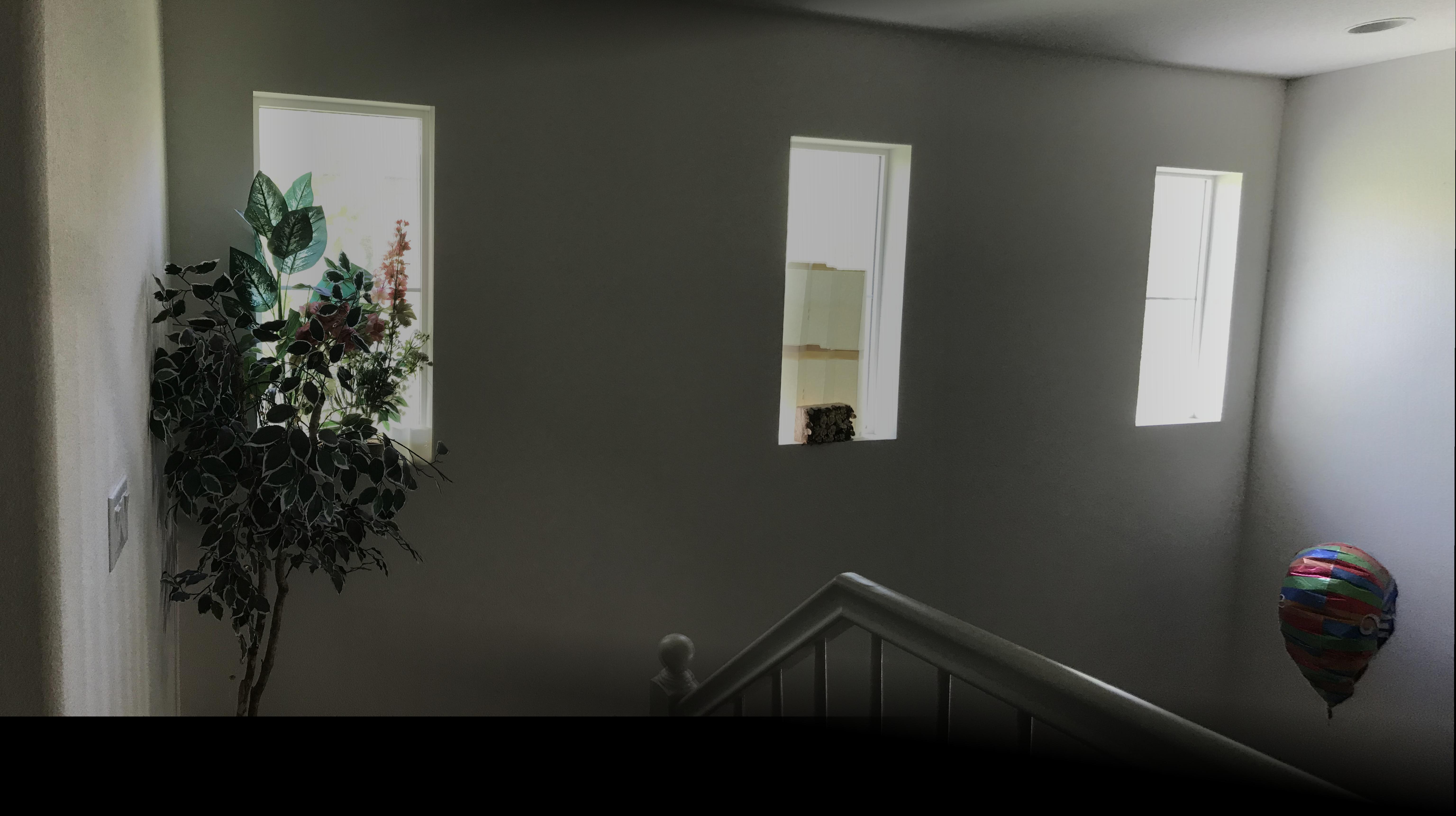 Wall: Mosaic
|
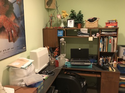
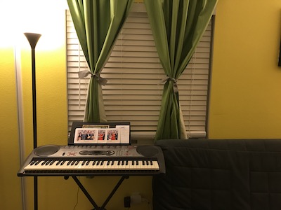 Room: Left
|
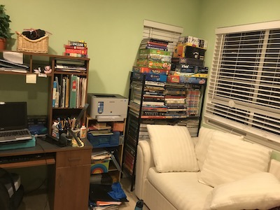
 Room: Right
|
 Room: Mosaic
|
 Loft: Left
|
 Loft: Right
|
 Loft: Mosaic (Failure Case)
|
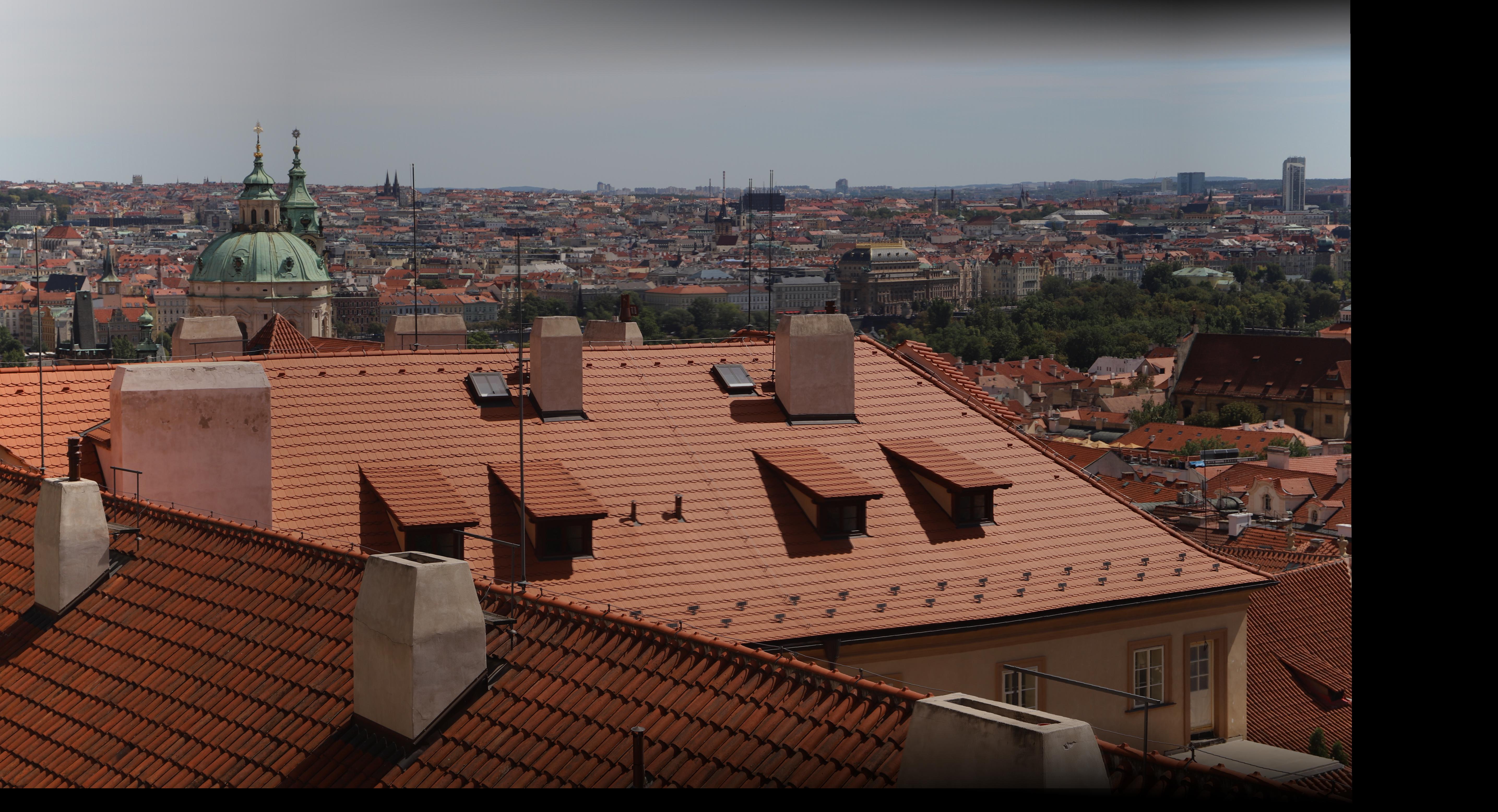
 City: Left
|
 City: Right
|
 City: Mosaic
|
In particular, the loft panorama turned out incredibly stretched, most likely
due to how I took the pictures. Since I was standing in the center of the room,
and pivoted in a circle to capture the images, it caused the resulting panorama
to not really account for that rotation, and stretch out the sides instead to
account for this. Due to this, I made sure to take into account this when taking
the rest of my images for future reference.
What I learned
In this part, I learned how simple it was to rectify things, only needing to use a
simple least squares formulation, and how I could create cool panoramas just using
techniques I used from previous projects! It was really interesting how everything
built together to create these new images, and its exciting to see how the underlying
technology for doing these sorts of things is actually remarkably simple.
Part B: Feature Matching for Autostitching
In the previous part, I manually defined correspondence points in order to find the
appropriate homography; this time however, the goal was to figure out how to implement
automatically finding the homography, in order to create a better and automatic matching.
For the subparts, I demonstrate the intermediate results on my wall images, although
I eventually use this automatic matching technique for all the same previous mosaics!
Step 1: Corner Detection
In order to first detect corners, I used the provided harris.py code, and ran it
on both of the two images that I wanted to combine. Essentially, the code returned
a set of interest points, or Harris corners, from each image, as well as their individual
corner strength. I also used a minimum distance of 35 pixels between the corners in order
to create more spread between the corners, since I had relatively high resolution images
and I didn't want too many points. Below are the results of plotting these Harris corners
on each of their respective images:
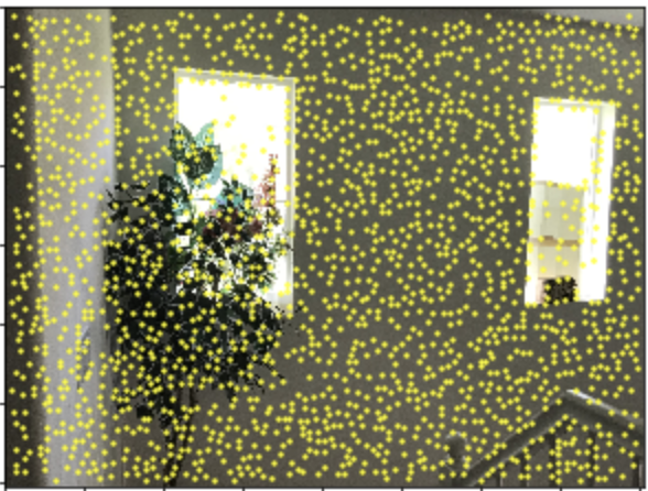 Left: Harris Corners
|
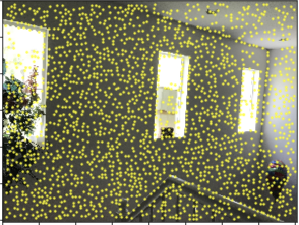 Right: Harris Corners
|
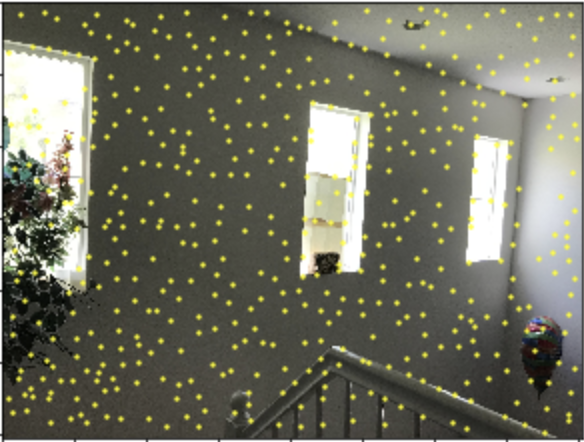
Next, I implemented Adaptive Non-Maximal Suppression, which resulted in taking a
sparser subset of these chosen corners in order to be more selective with our
desired matches. Basically, ANMS works by going through all the provided Harris corners
and checking each one for its minimum suppresion radius. I computed for each corner
the closest other corner that 'suppresses' it, which means the closest one that meets
the criteria where its strength times 0.9 was still greater than the current corner's
strength. Doing this allowed me to reduce the thousand over Harris corners given to a smaller
subset of 500 per image, as seen below:
 Left: ANMS
|
 Right: ANMS
|
Step 2: Feature Descriptor Extraction
Next, for each of my remaining corners, I took that corner as the center of a
40 x 40 pixel box, and downsampled it to 8 x 8 with a stepsize of 5. Then I
demeaned and normalized this box to get a generic descriptor of the corner.
Essentially, this method allows for similar features to map to boxes with
similar SSD values, which will be helpful later for feature matching. Below
are the display results of one of the descriptors from each image. Note that
the descriptor is resized visually up from 8 x 8:
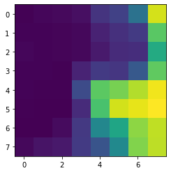 Left: Feature Descriptor
|
 Right: Feature Descriptor
|
Step 3: Descriptor Matching
To determine which of the features in each image were good matches for each other,
I took the SSD of each feature descriptor in one image with each feature descriptor
in the other; then for each, I obtained both the first nearest neighbor (1-NN) amd the
second closest nearest neighbor (2-NN). By Lowe's rule for thresholding, I concluded that
I could choose to only include feature pairs that whereby the ratio between the first
and second nearest neighbors were less than 0.5. Essentially, what this meant is that
the SSD to the 1-NN was a lot smaller than the SSD to the 2-NN, which meant that the original
two were very likely to be correct and matching correspondence points. This was just outlier
rejection, and allowed me to throw out a large amount of points that did not have good
correspondences with other points. Then to tidy up the remaining points, I also removed
duplicate pairs that existed from checking the threshold in both directions.
Step 4: RANSAC
With a bunch of pairs of corners between the two images, I then used 4 point RANSAC to
create a better homography estimate. The procedure for this is to arbitarily select four
pairs and compute the homography transformation between them, exactly rather than using
least squares. Then, I went through all pairs of points (p, p'), applied the homography tranformation H
to p, and then took the SSD between Hp and p'. If this SSD was less than 1, I concluded that the
correspondence points matched the transformation, and added it to a current set of inliers. Doing this
for a long time, about 10000 iterations, and then taking the largest set of inliers allowed me to decide
that the remaining set of inliers were highly likely to be correct correspondence points. The last step
of RANSAC is to then compute the least squares homography matrix over all the inliers, which in turn created
a more accurate estimation.
Step 5: Run Original Alignment w/ New Homography
Using this automatically generated homgography matrix, I could then just run the
original alignment code to create mosaics and panoramas as before! Below are the results
of the same source images, as before, although on the left is the result of manual correspondence
selection, while on the right is the result of automatic stitching:
|
Manual
|
 Automatic
|
|
Manual
|
 Automatic
|
|
Manual
|
 Automatic
|
|
Manual
|
 Automatic
|
The automatic stitching appeared to better correct the alignment between both
the city image and the loft image! Overall, the mosaics made appeared to be of
a higher quality, and were more refined as a whole.
What I learned
The coolest thing here was how everything really came together to be able to create
these amazing panoramas automatically! It was really cool how the computer manages to
achieve similar or even better results than just the human eye automatically, even though
you would think that manually defining correspondence points is something that humans would
be better at doing. As a whole, this project was really rewarding, and I learned so much about
how we can use these techniques of feature detection and matching in order to automatically stitch!
Also RANSAC is really cool :')