Part 1

Overview

In this project, we first set out to use least squares to compute a homography matrix that allows us to warp one image into another.

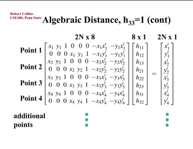(source: http://www.cse.psu.edu/~rtc12/CSE486/lecture16.pdf)

In order to warp an image into another image, I used an inverse warping technique. To do this, I first must calculate the set of all points in the destination image that map to the source image. As the warped image will still be a quadrilateral, we can create a bounding box by translating the corners of the source image using our homography matrix. Then we can use these corners to generate a superset of the necessary points.

With these points, we can translate them back to the source coordinate system using the inverse of the homography matrix we calculated going from the source image to the image we are warping to. With these newly translated points, we can delete any that went out of bounds of the original image. For the ones in bounds, we can simply grab the color at that position (or a lerp of surrounding pixels) and color the new warped image with the corresponding colors.

Results

Rectification

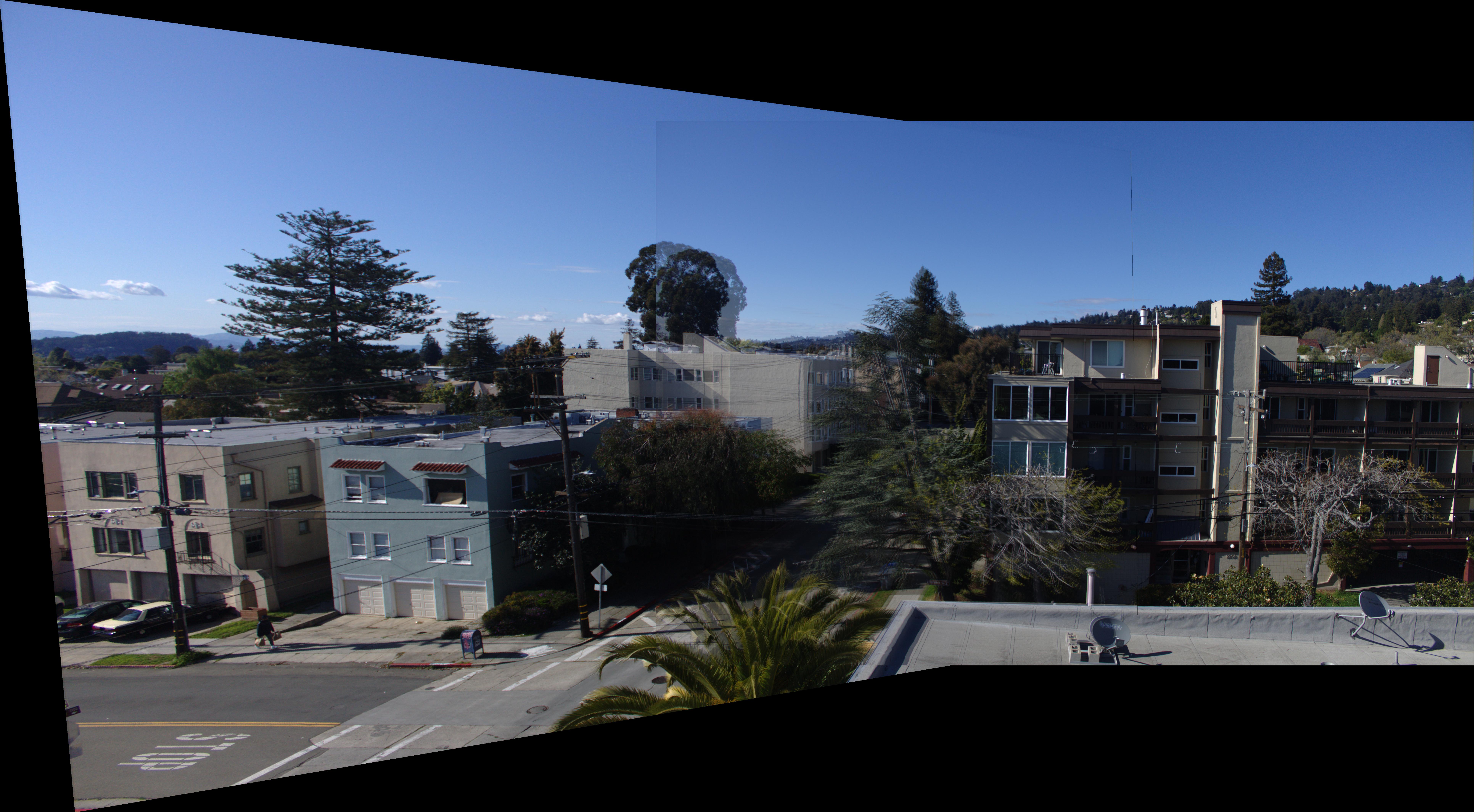
Here we can see how we can use this warping to rectify an image.

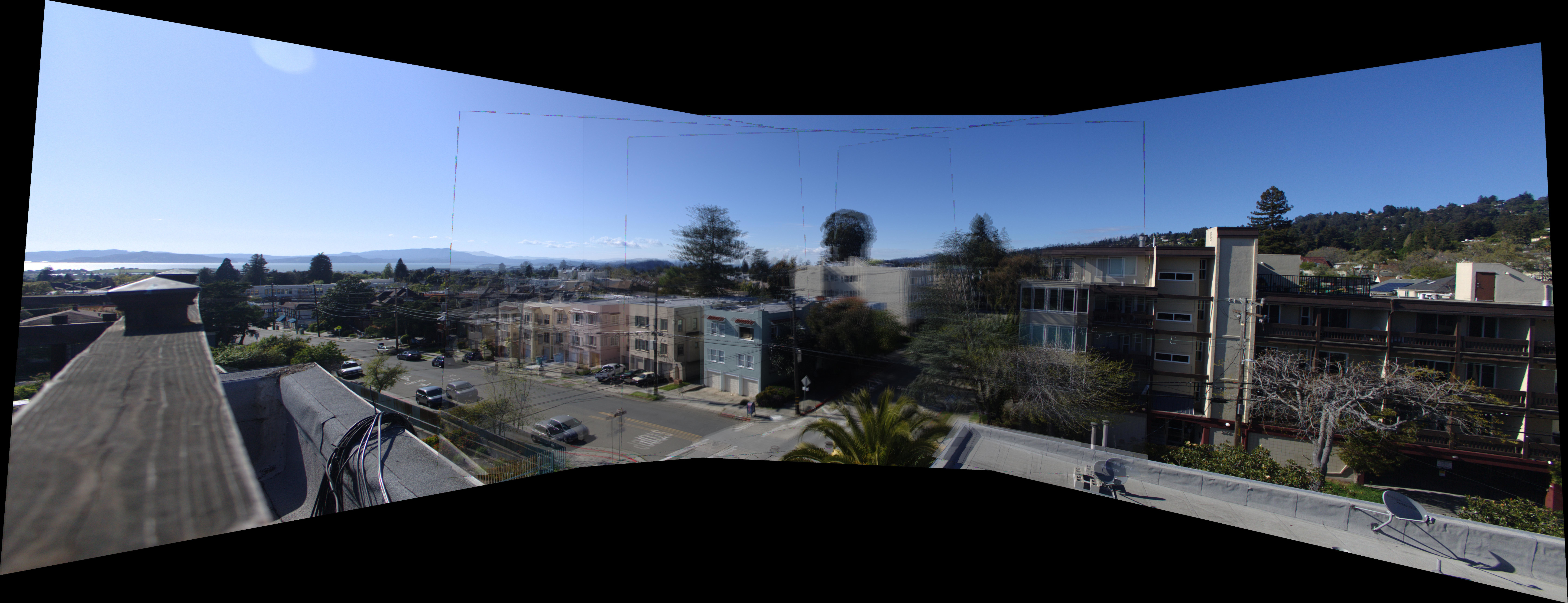
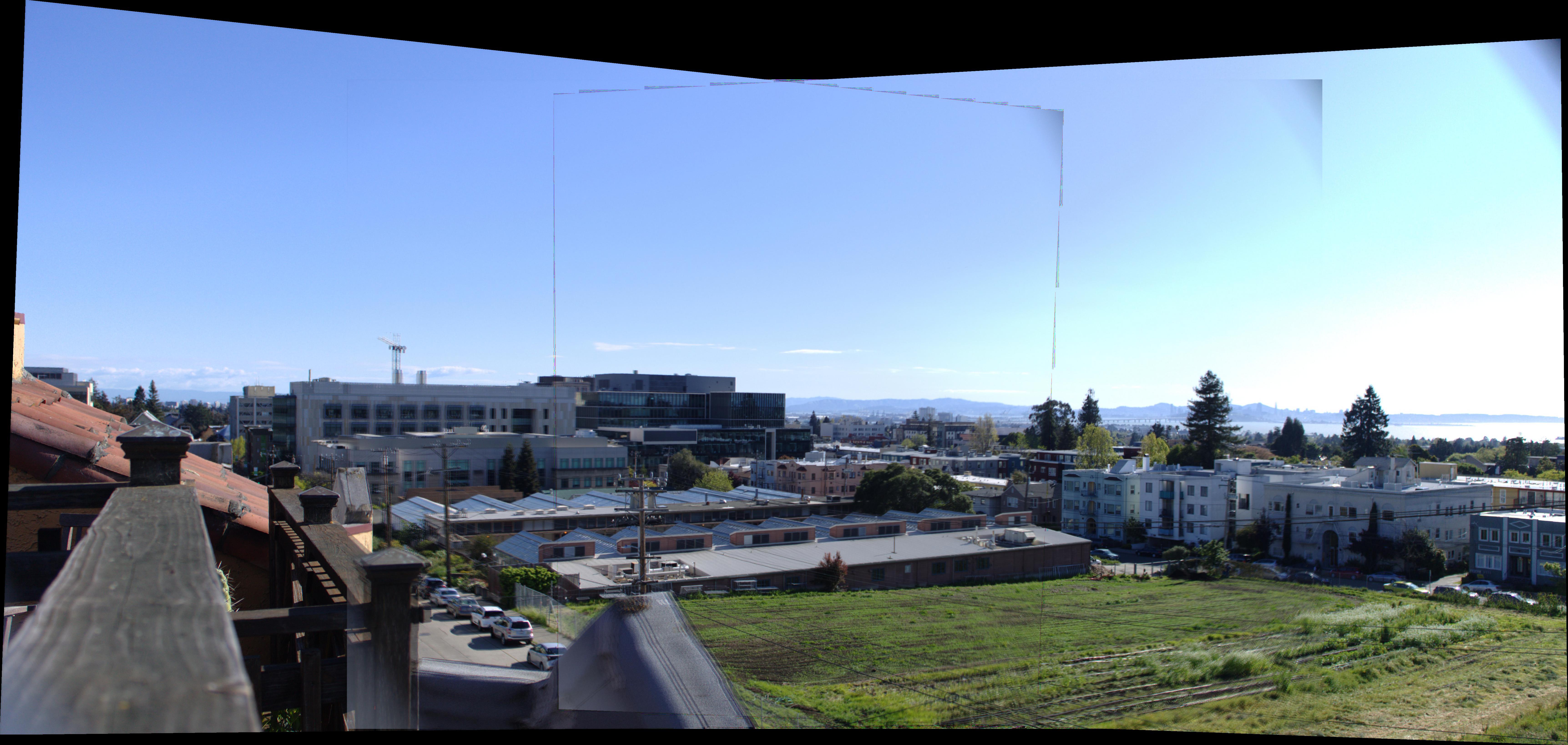
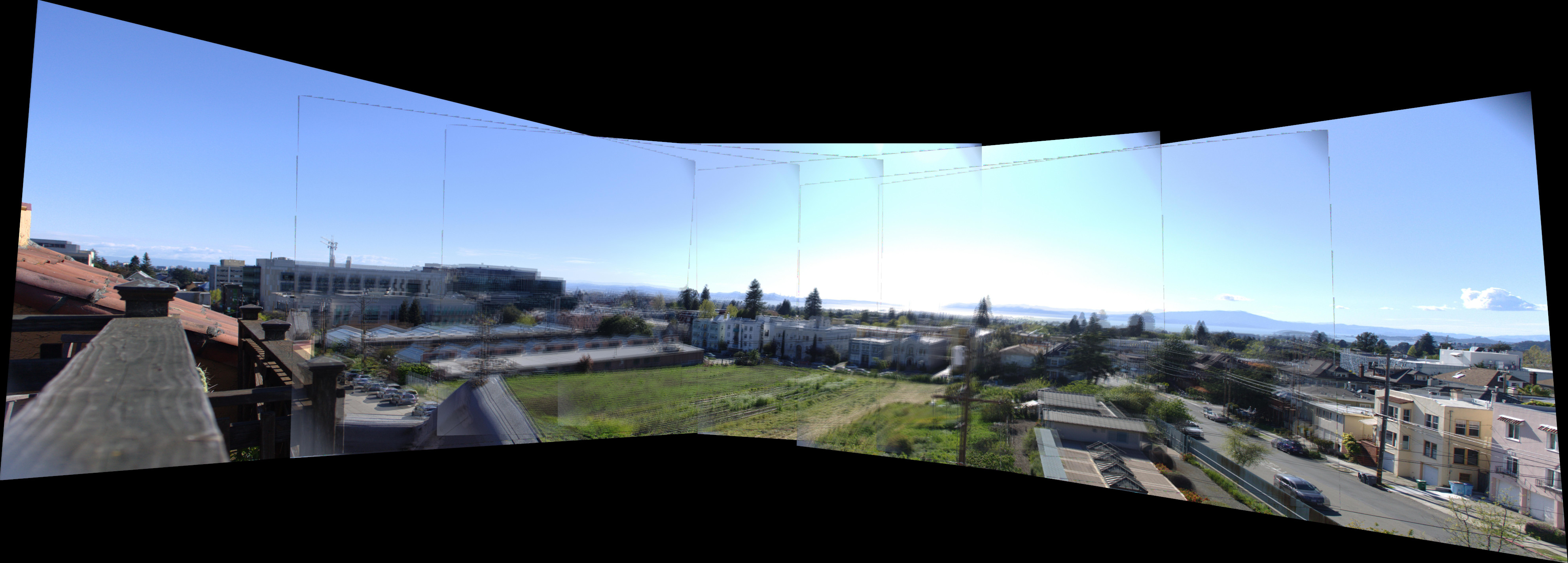
Stitch

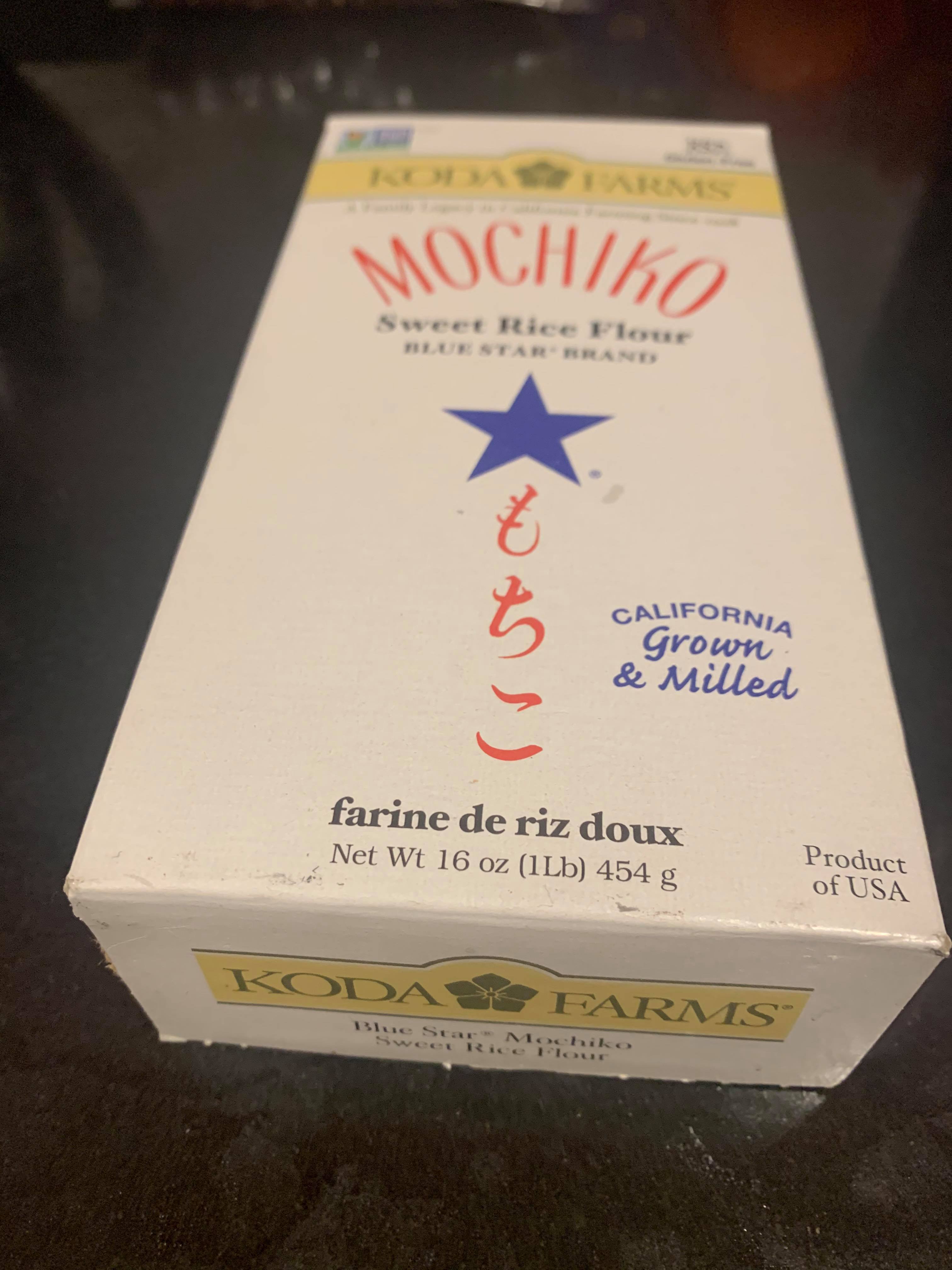
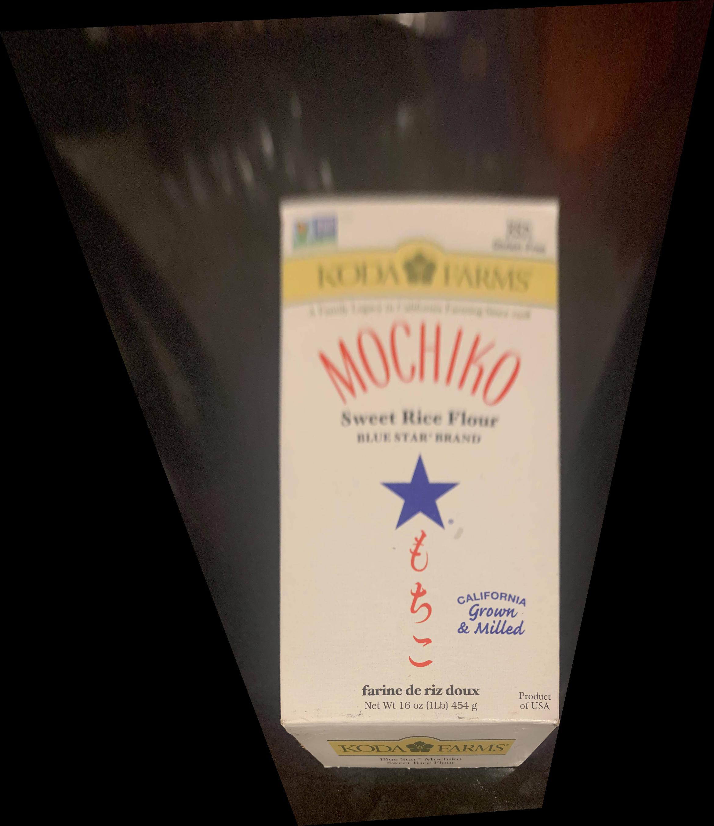
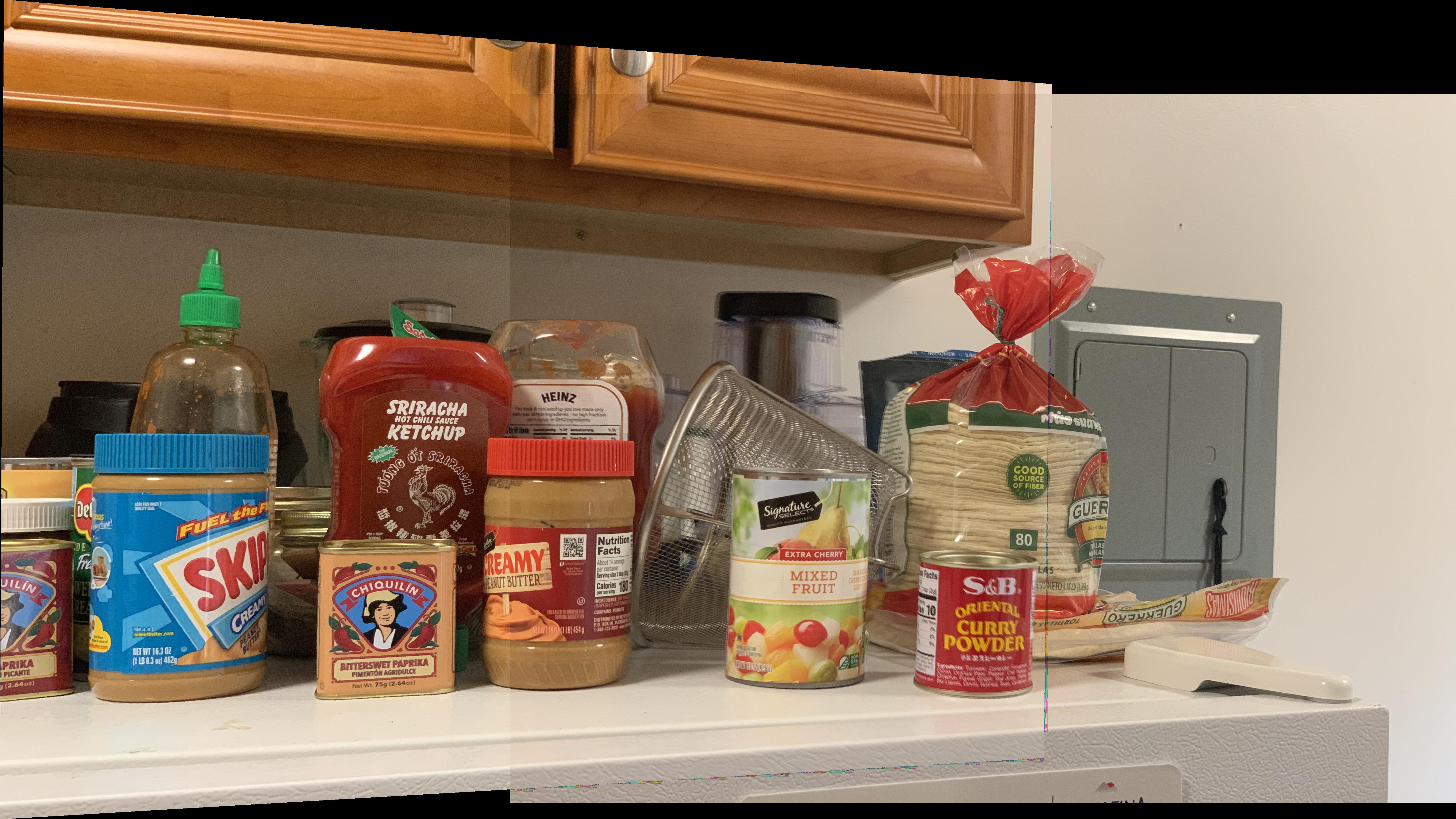
Mochiko

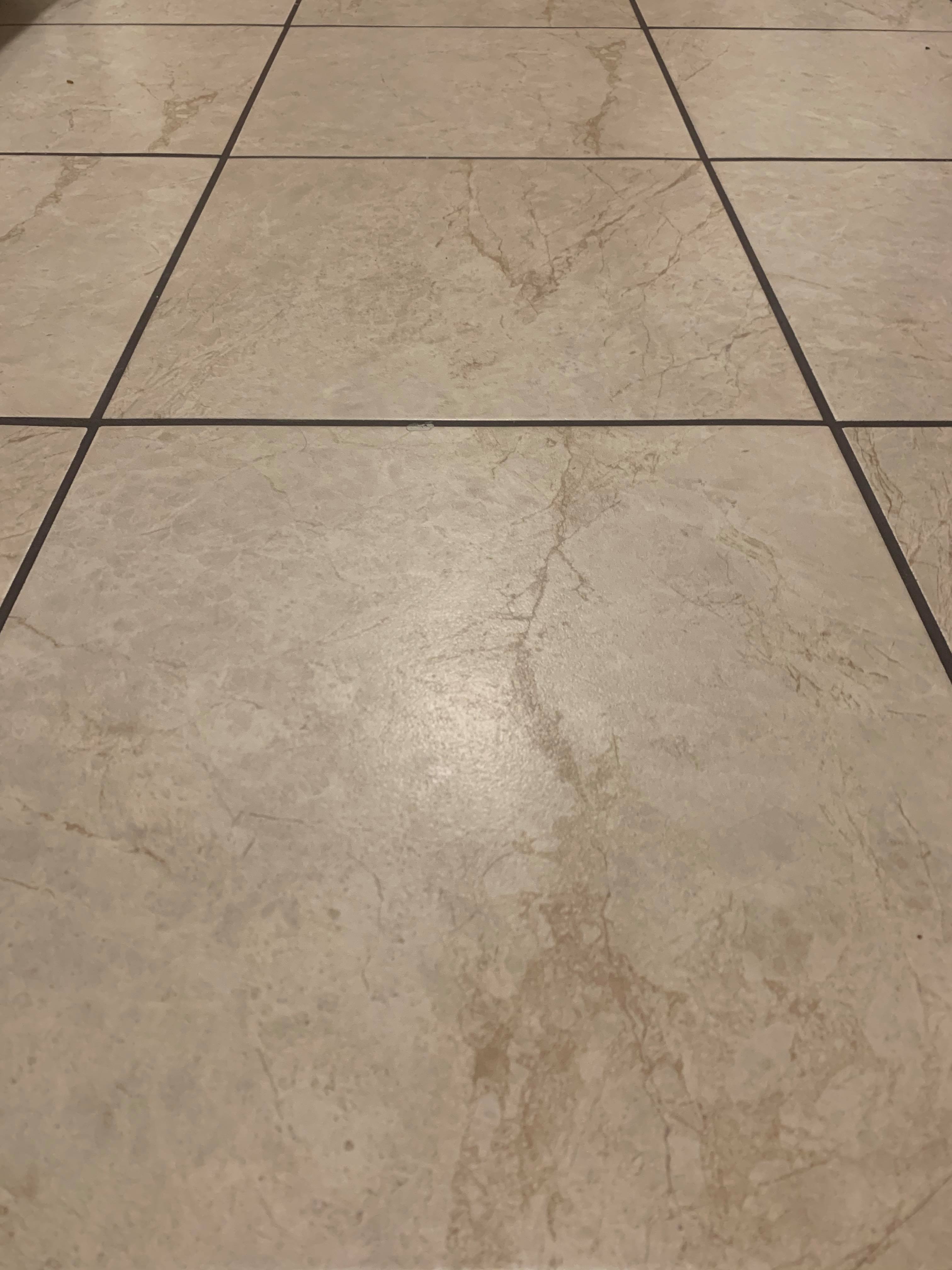
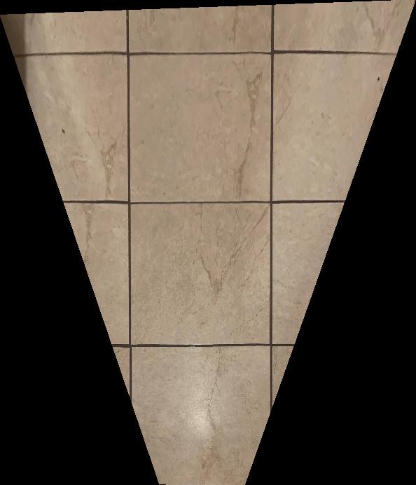
Tile Floor

Blending

We can also blend together images using this same technique but overlapping the images.

Conclusion (part one)

In this first part of the project, I really enjoyed blending the images and creating panoramas. I learned about how to think about the images as a change of basis of coordinate systems and this helped me greatly.

Part 2

Overview

As selecting correspondencies is very tedious, time intensive, and error prone (as being off by a few pixels creates somewhat “shaky” blends like the one above), the next part of this project aims to automate this by generating possible features, matching them between images, and then using the RANSAC algorithm to discard outliers.

Harris Corners:

Using an edge_discard factor of 40 to ensure adequate padding for feature extraction, I got approximately 5000 harris corners for my testing images.

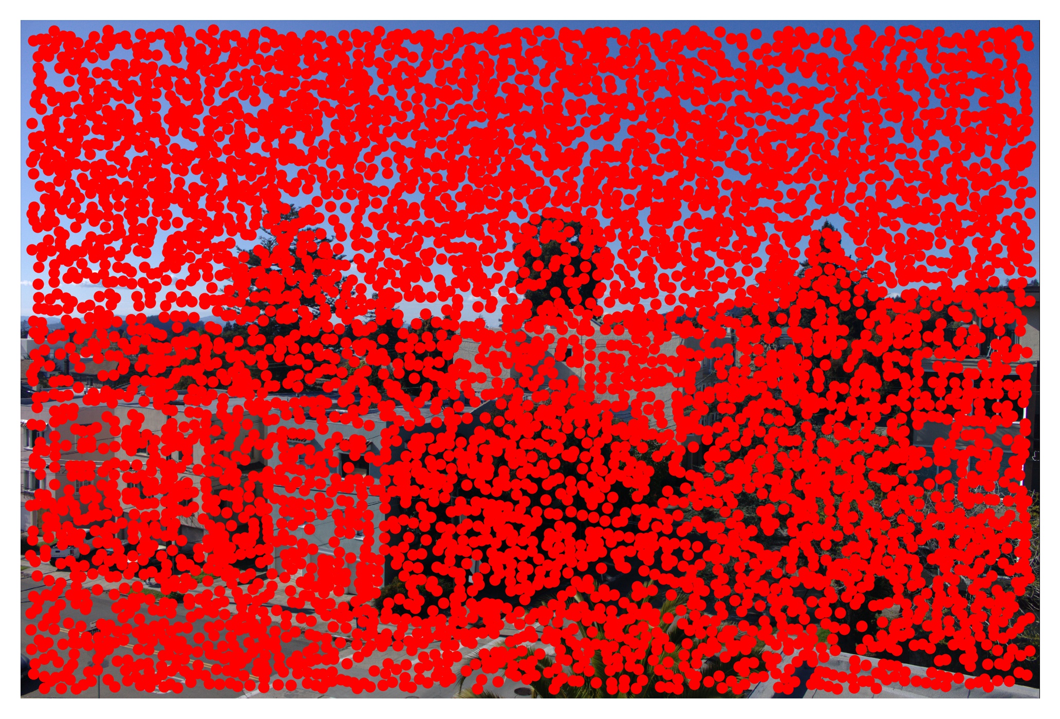
As this is obviousally too many points and not all of them will be meaningfully able to be matched to another image. I could tune this down to be lower (as seen in the following photo) changing a few parameters of the harris functions but did not do that as the next step (ANMS) will prune out values to be an appropriate amount.

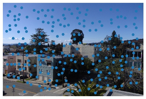
Adaptive Non-Maximal Suppression (ANMS)

To filter these points we can use the ANMS technique to chose a set number of well spatially distributed points. Choosing the top 500 of the ones above:

As we can see this is a bit more of a reasonable amount of points to work with and they seem to be on some decent corners of objects.

Feature Extraction and Matching

I extract 8x8 features into a vector of length 64 with mean 0 and std dev 1 from a 20% scaled version of the photo in order to generate a vector that we can use to compare with other images to match these features. To match we calculate the Euclidean distance from each feature vector in one image to each feature vector in the other image. Then, we can look at these distances and choose the two closes features in the other image. If the ratio of the distances between thes two is under some threshold, then we can use it a potential match between the two images.

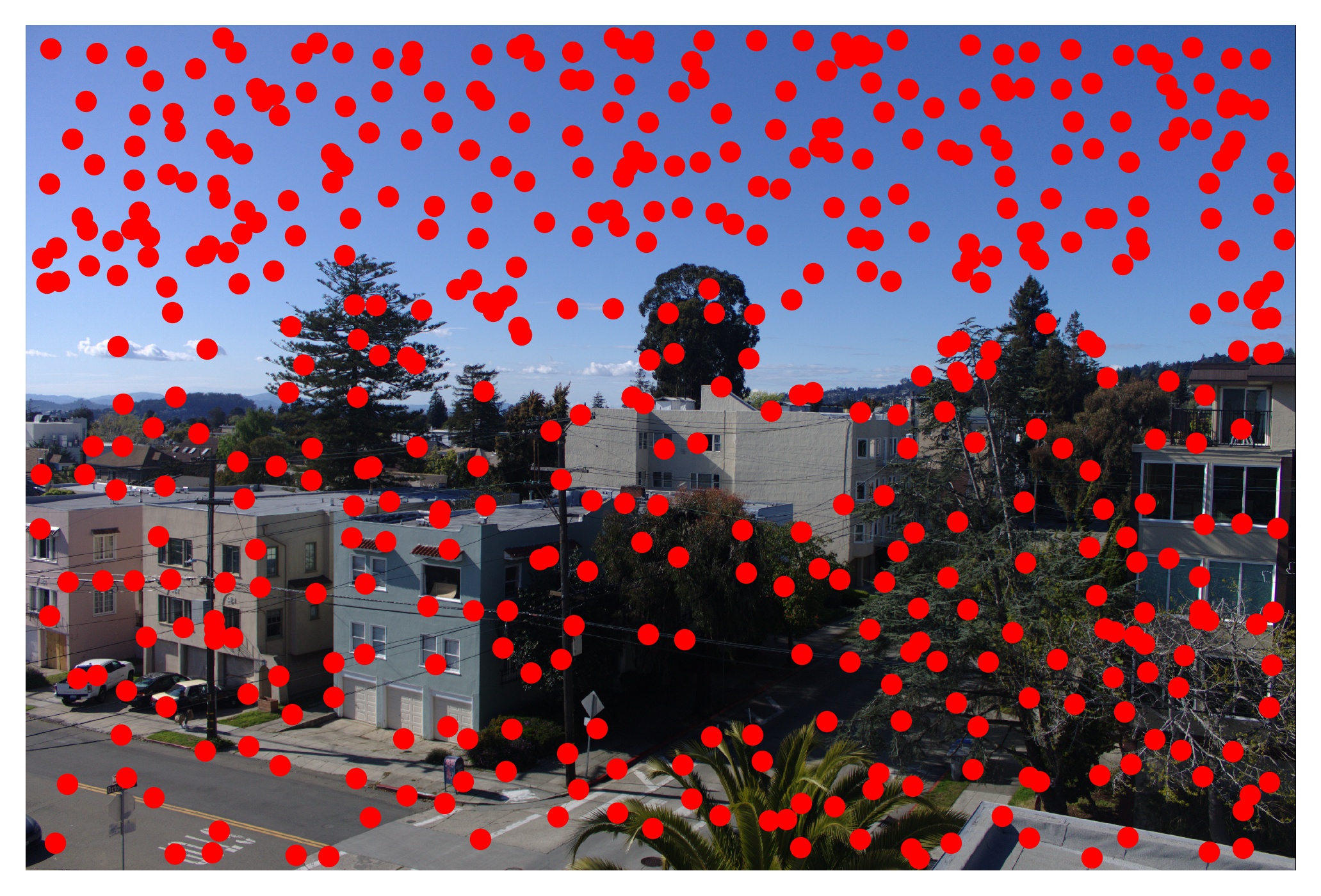
As we can see this worked reasonably well and there are indeed some decent matches, but there are also some outliers that prevent these points from being used to generate a good homography.

RANSAC

To remove the outliers in the last step, I ran 10000 iterations of RANSAC with a threshold of 0.15 and four samples per iteration. This means that I grabbed four random correspondences, calculated the homography between them and then mapped all correspondencies using this homography matrix. I then counted the number of points that the homography mapped close enough to the potential corresponding point in the other image (this is the number of inliers). I then found the maximal set of inliers doing this and used those to calculate my final homography matrix.

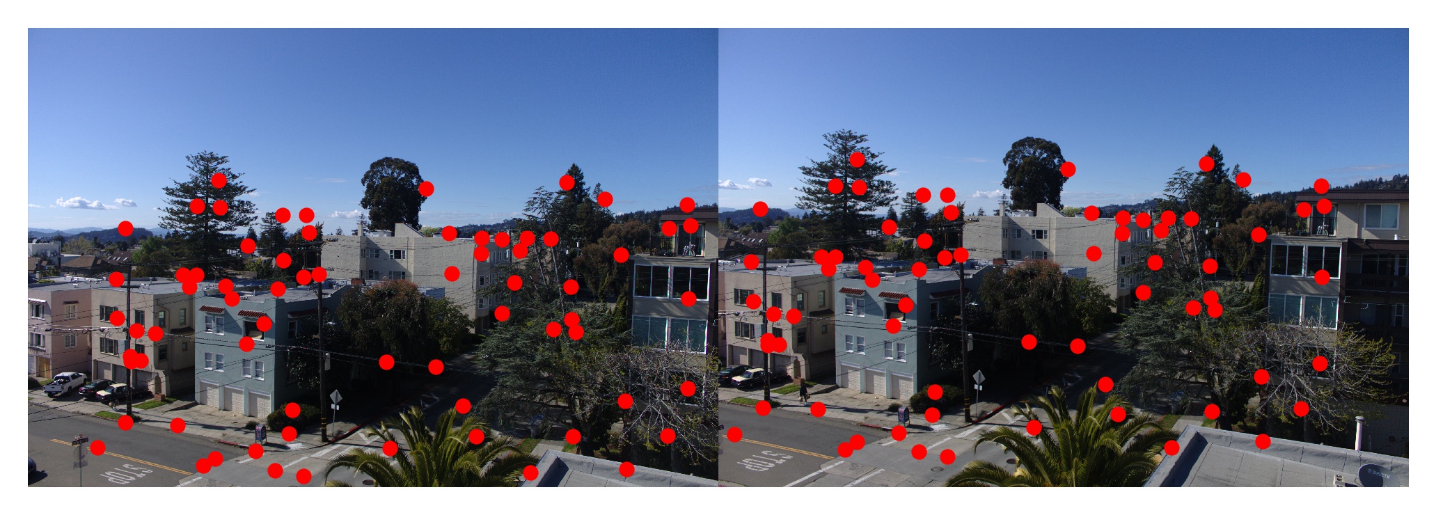
This image represents the final correspondences that RANSAC generates at the end of the algorithm.

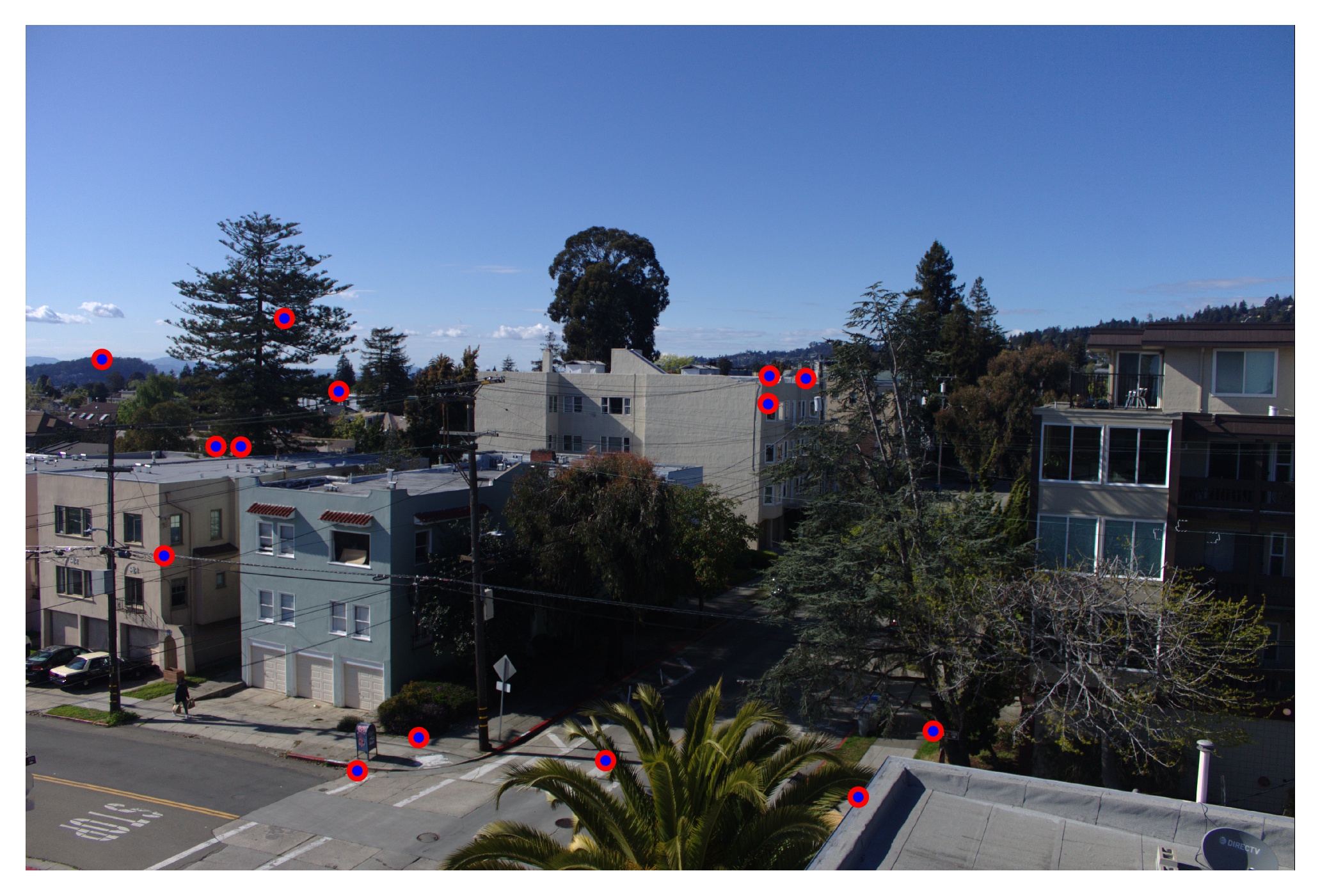
This image represents the points mapped by the final homography generated by RANSAC in blue and the harris corners of the corresponding points in red. As we can see, they match very well which should help us generate a good homography.

Auto stitching

Using this, we can easily generate correspondence points and autostitch images!

We can see the improvement on the same two blends from above:

Manual Correspondences	Auto Correspondences

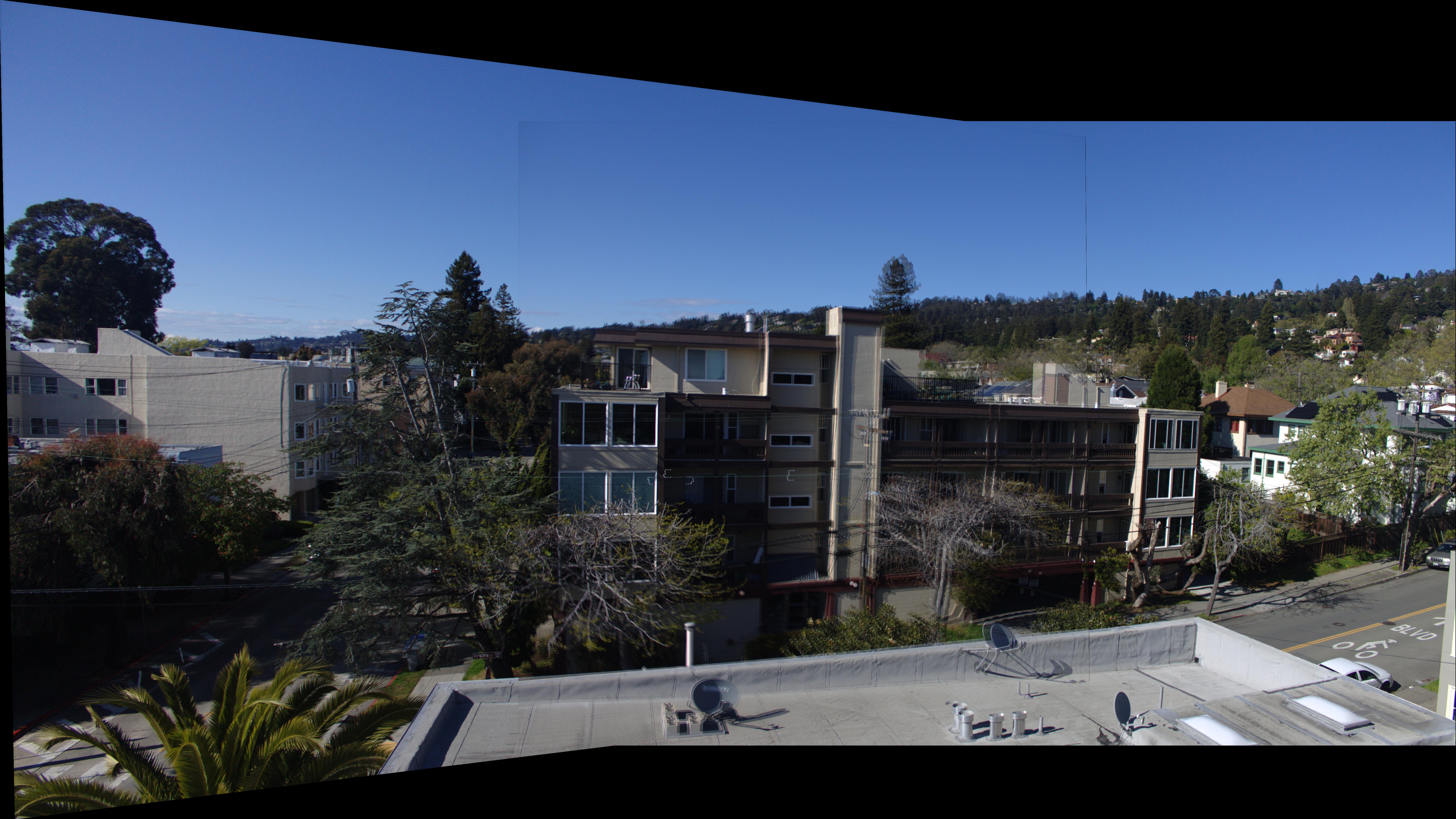
As well as on the larger full panorama:

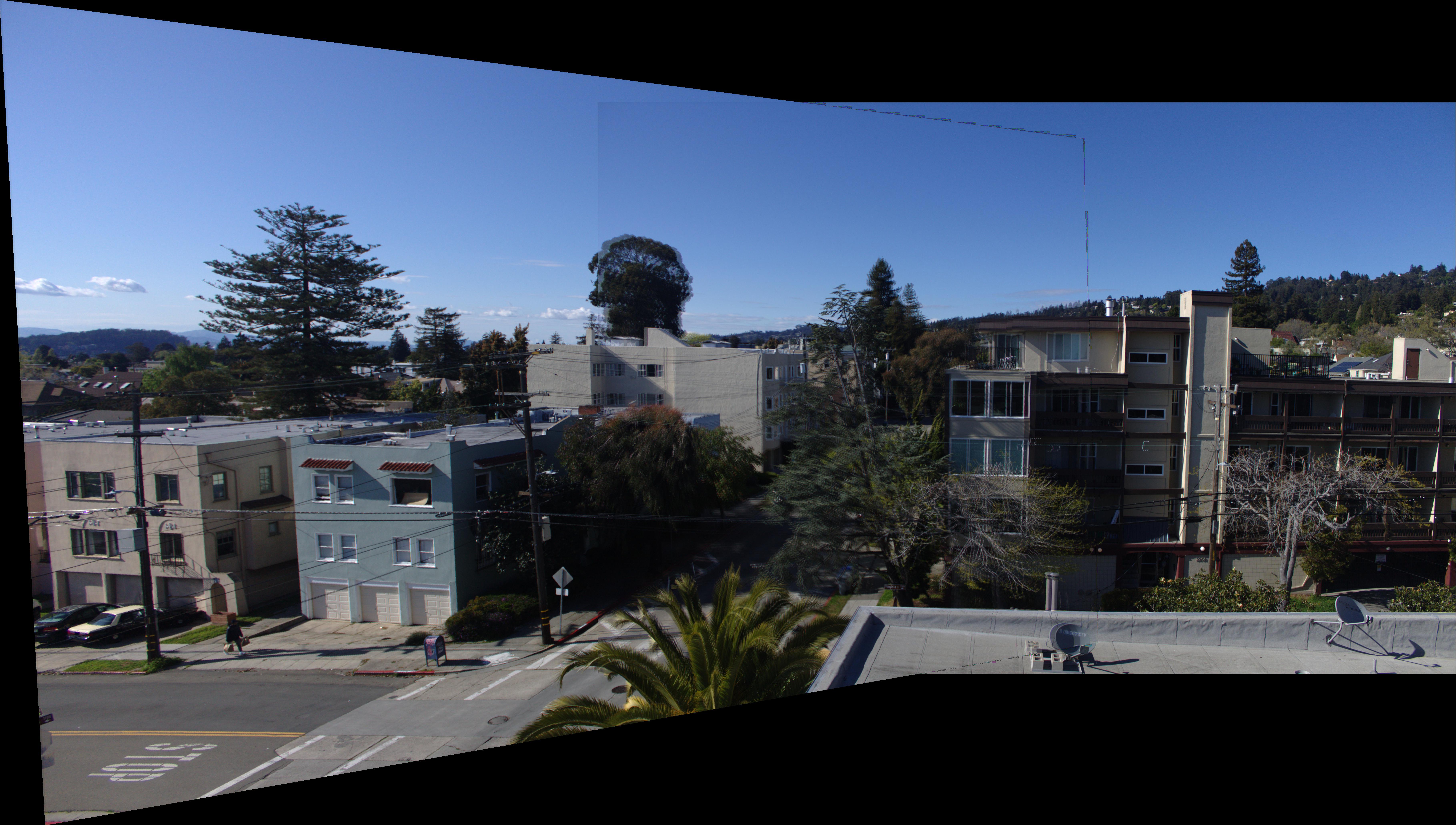
Manual Panorama:

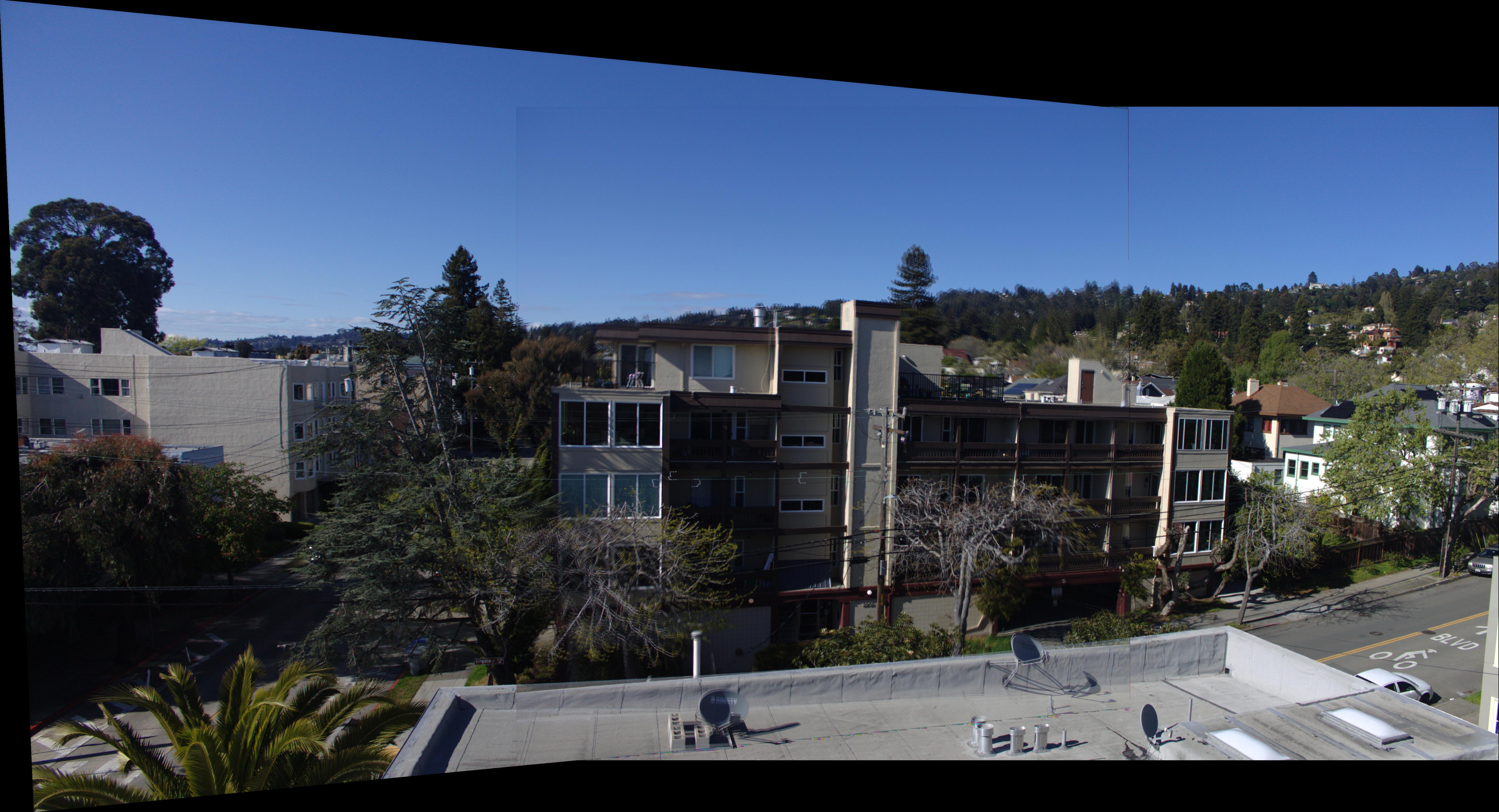
Auto Panorama:

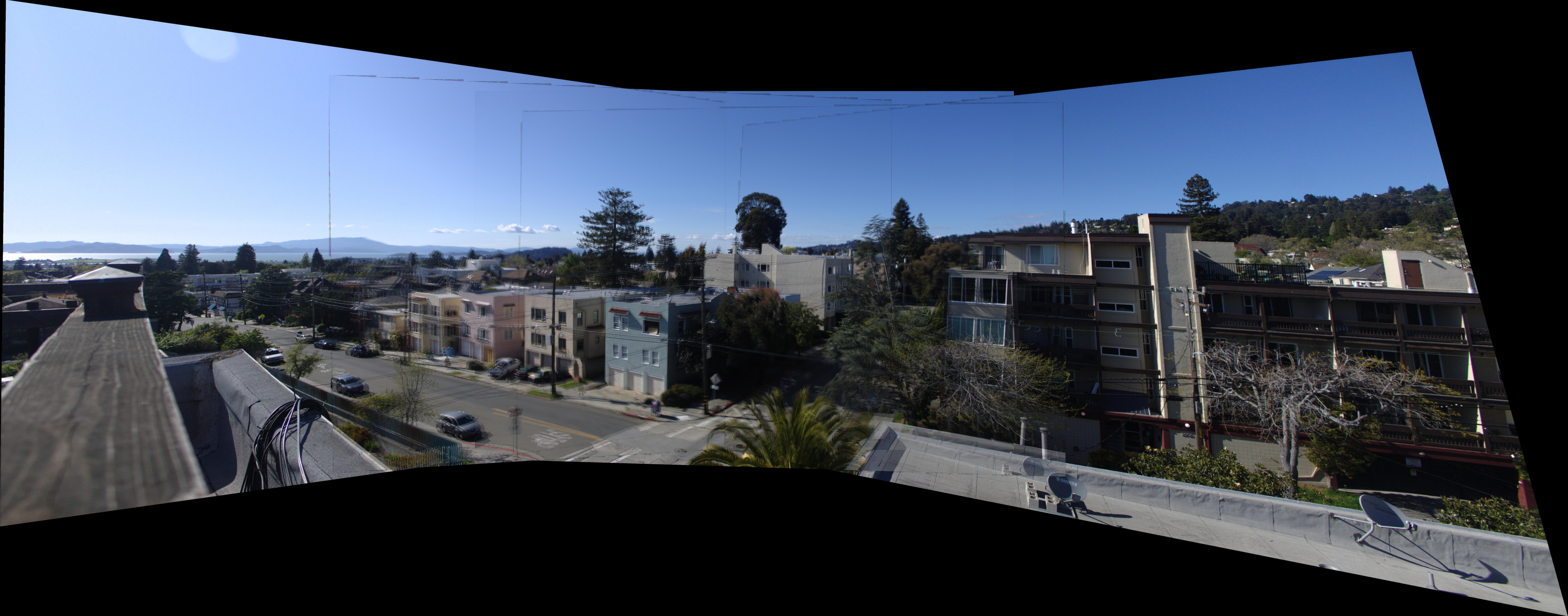
As we can see due to the larger number of and more precise correspondence points (the manual only had 8 per image pair), the auto stitching works much better than manual stitching while being much less tedious!

More panoramics:

Conclusion (Part 2)

I really enjoyed learning about how we can use something as simple as corner detection to generate a list of correspondences. The statistical feature matching and filtering to make a robust set of correspondences was very interesting. I also enjoyed learning a lot of new techniques to manipulate numpy arrays to avoid having to do large for loops in Python.