In this project, we will take two or more photographs and create an image mosaic by registering, projective warping, resampling, and compositing them.
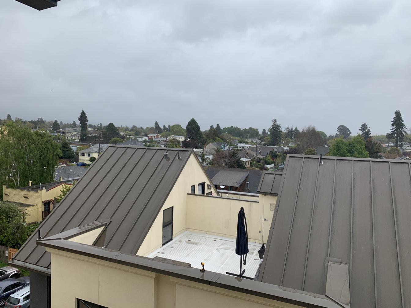
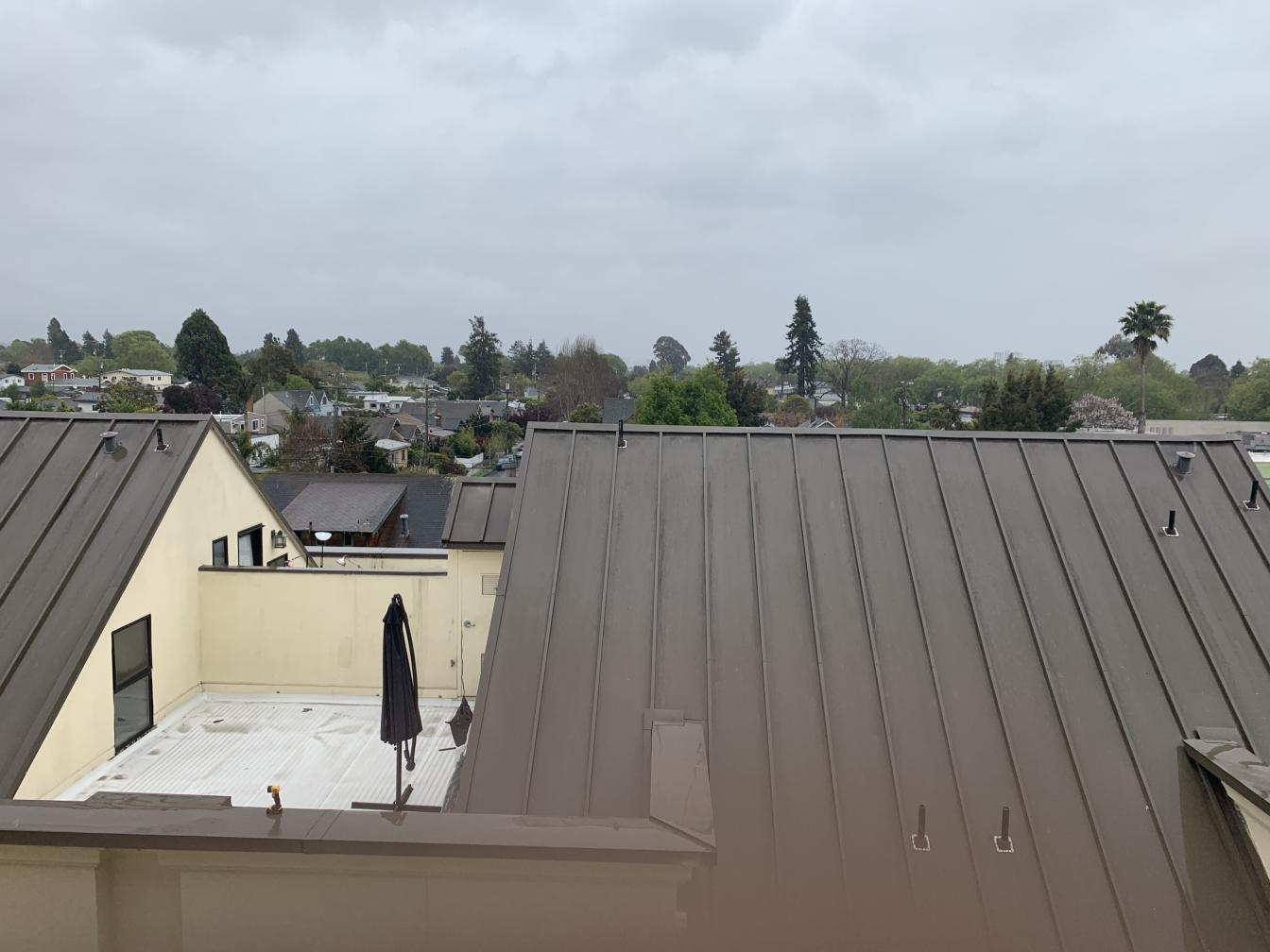
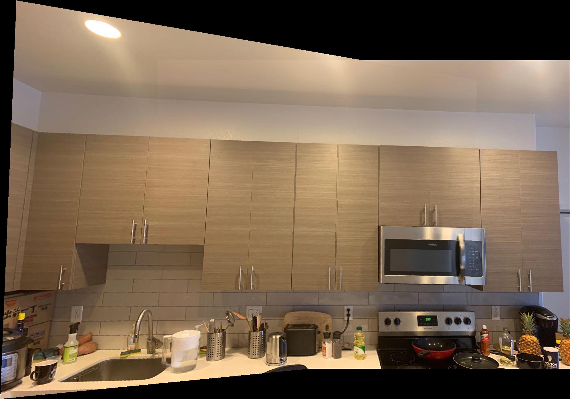
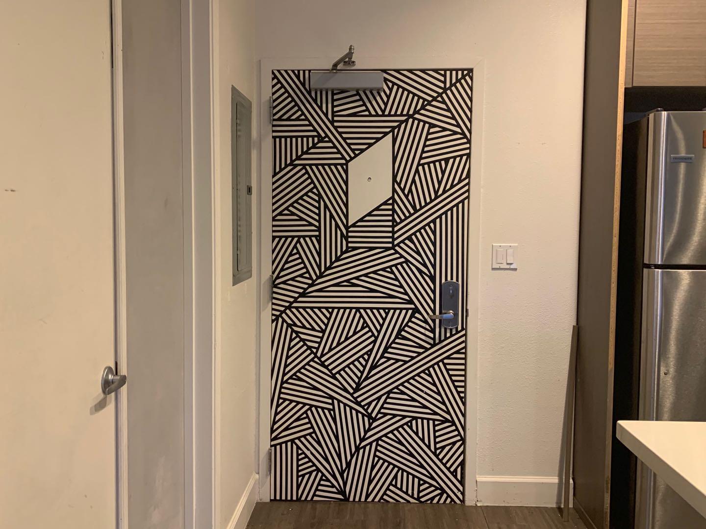
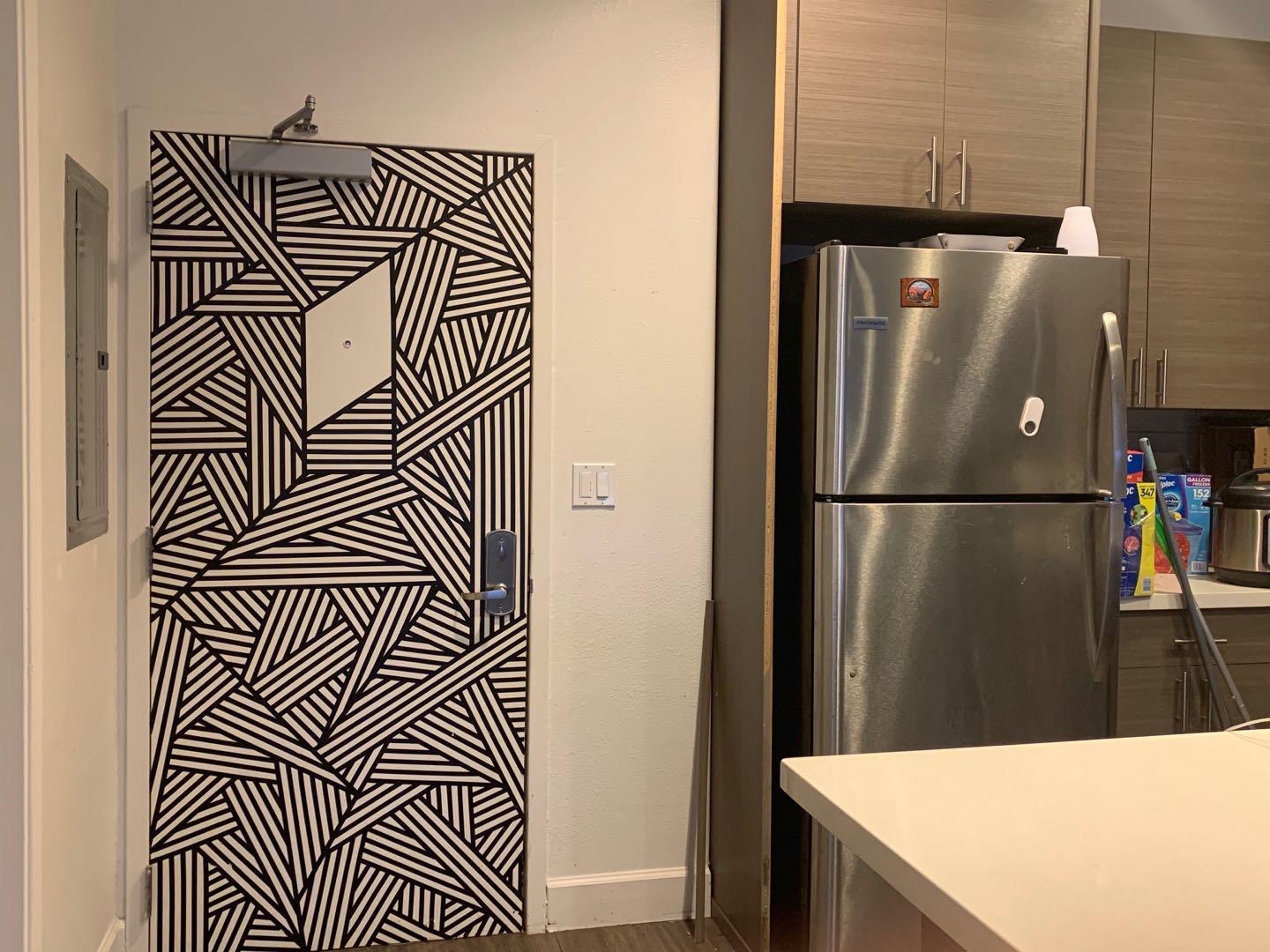
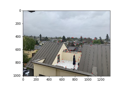
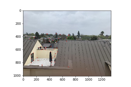
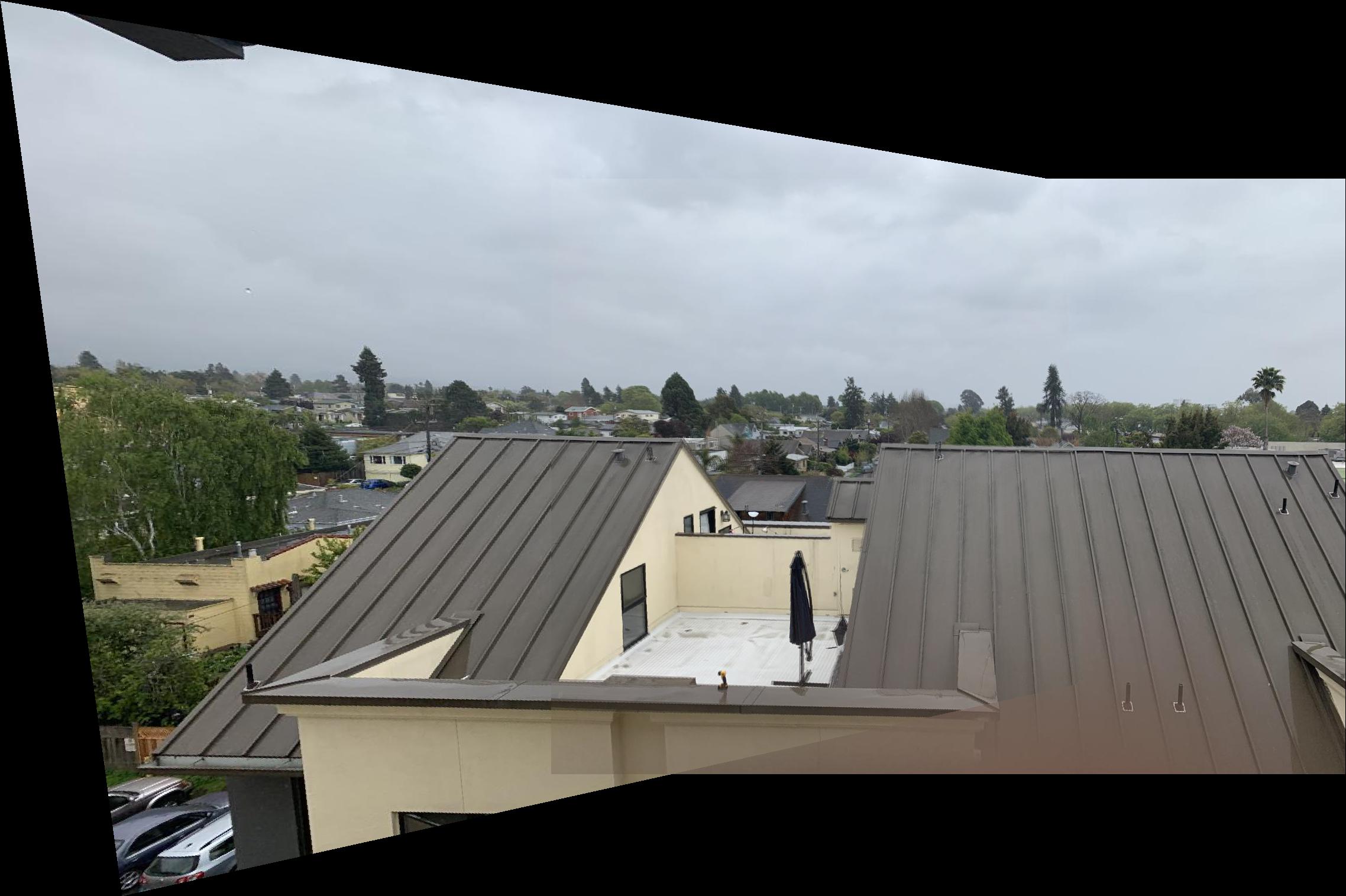
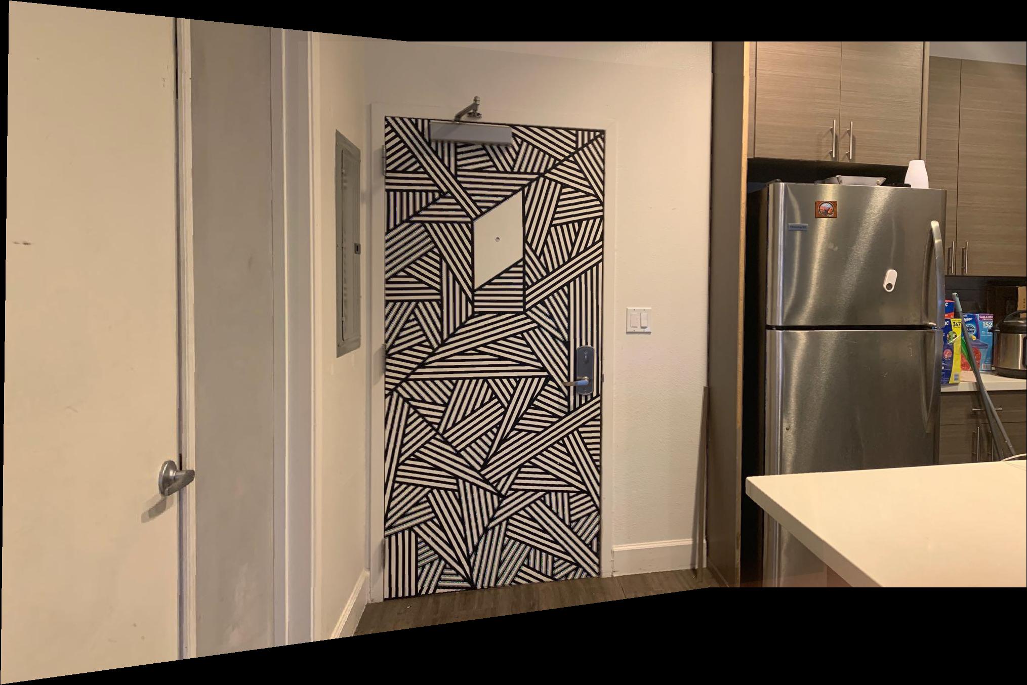
I shot pairs of photos from the same point of view but with different view directions and overlapping field of view. Images from my phone camera has a resolution of 4032 * 3024. To reduce computation, I downsampled images by a factor of one third. Here are some example images.
| Image 1 | Image 2 |
|---|---|
|
|
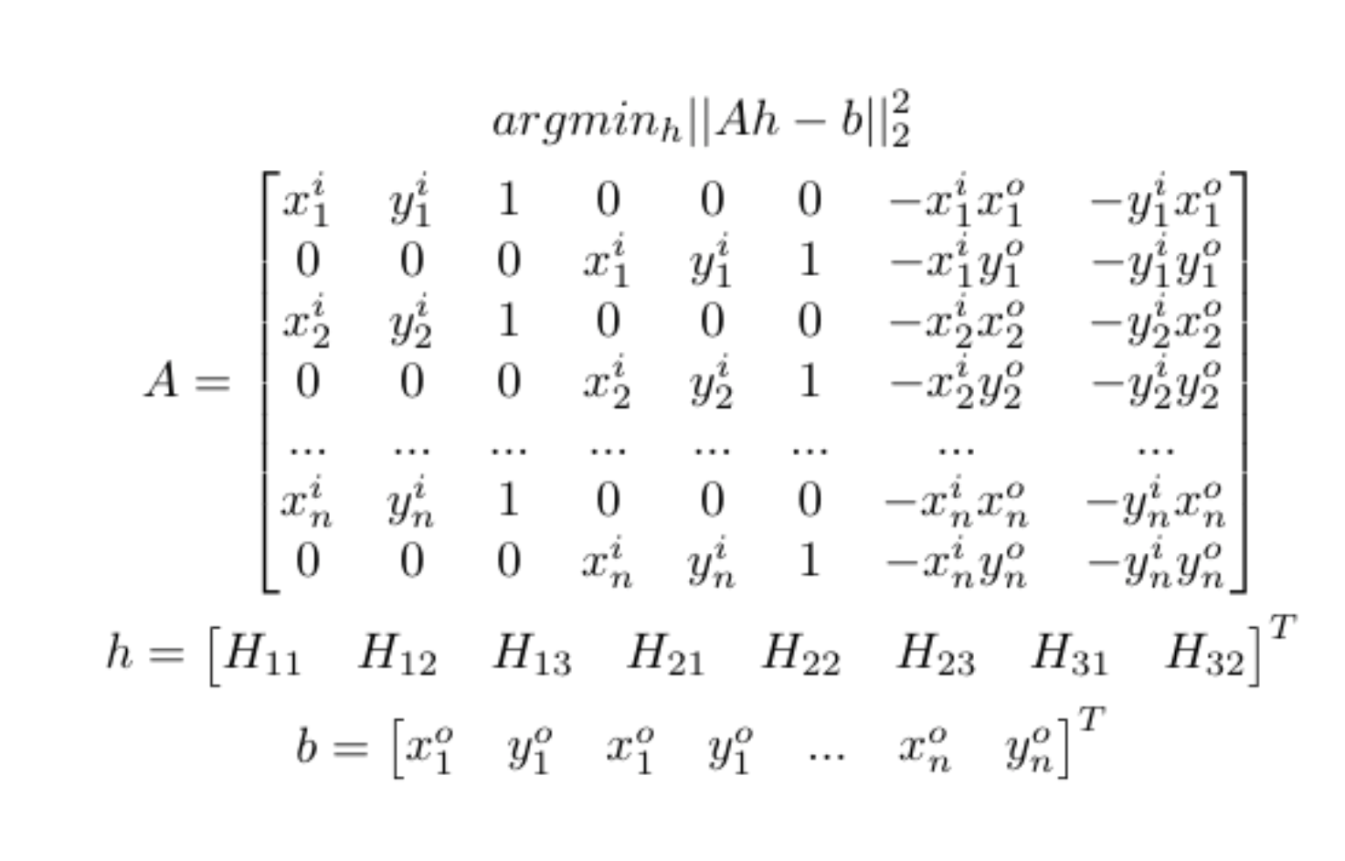
Denote H as the projective transformation matrix, we want to recover such H that x’ = Hx where H is a 3-by-3 matrix with 8 degrees of freedom. One way of solving the problem is to solve the following least square problem. In the following formula, superscript i stands for input and o stands for output.
 |
To warp the images, we use inverse warping to avoid any noticeable artifacts. The main idea is very similar to the that of project 3: used skimage.draw.polygon to get the (x,y) coordinates to and apply inverse warping to all coordinates. Also, I defined a helper function to generate a blank canvas for the resulting images and the proper offsets of x and y coordinates to avoid any negative coordinates.
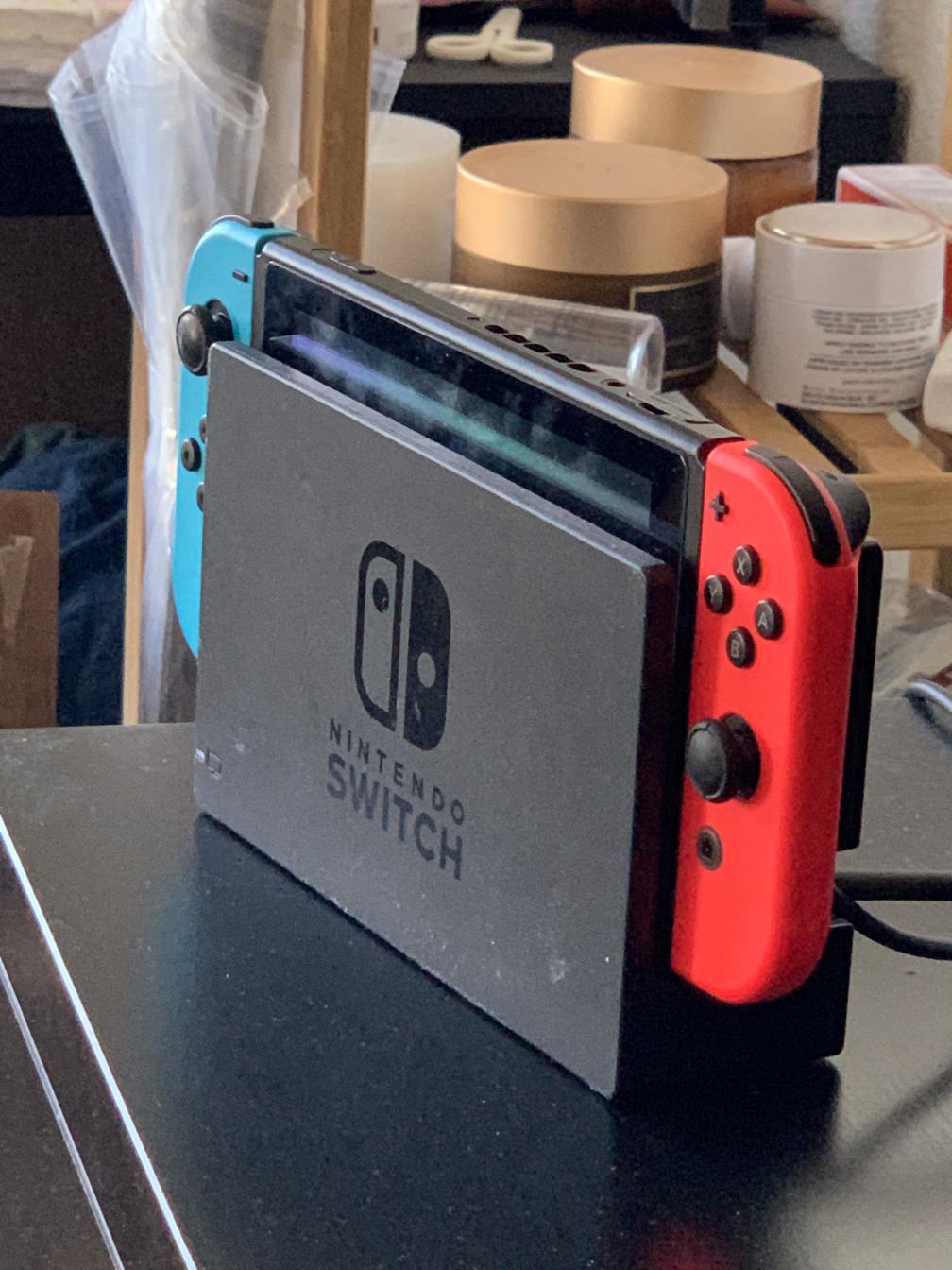
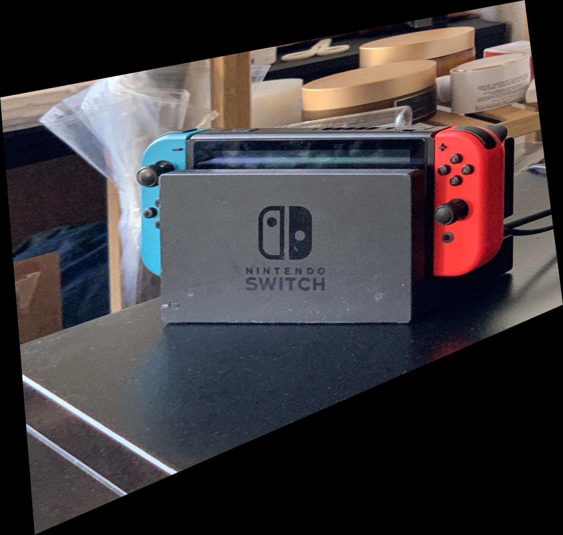
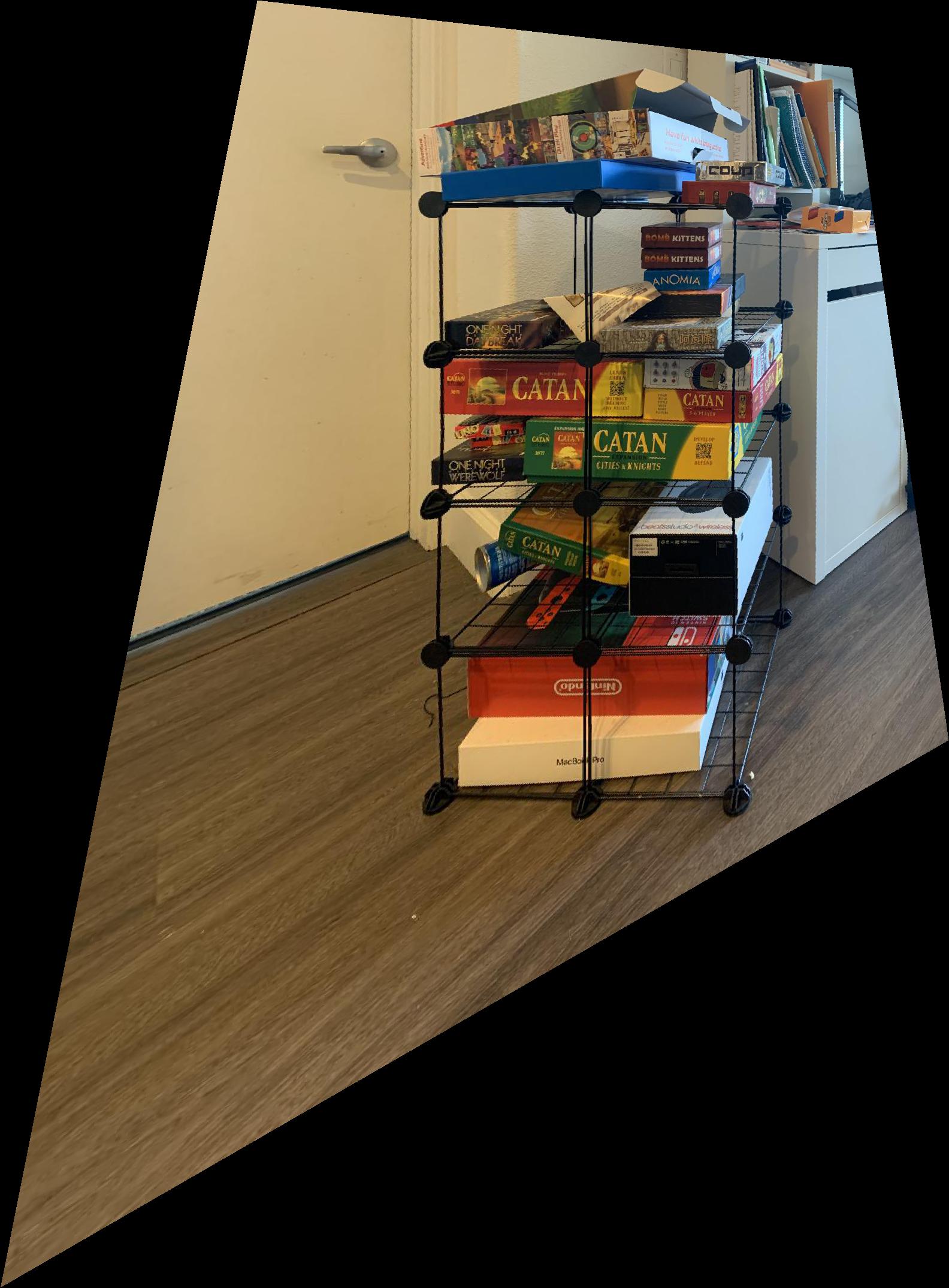
In the following examples, images themselves contain certain grid structure (corners for the shelf and Switch console). By selecting those points as correspondence and defined output points carefully, I was able to rectify those images.
| Original Image | Correspondence | Output Image |
|---|---|---|
 |
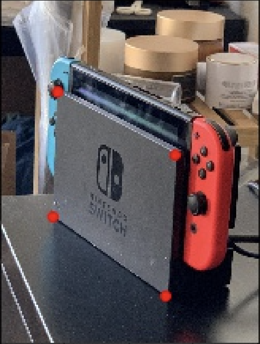 [0,0], [0,510], [860,510], [860,0] |
 |
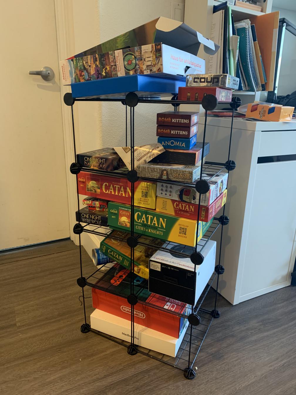 |
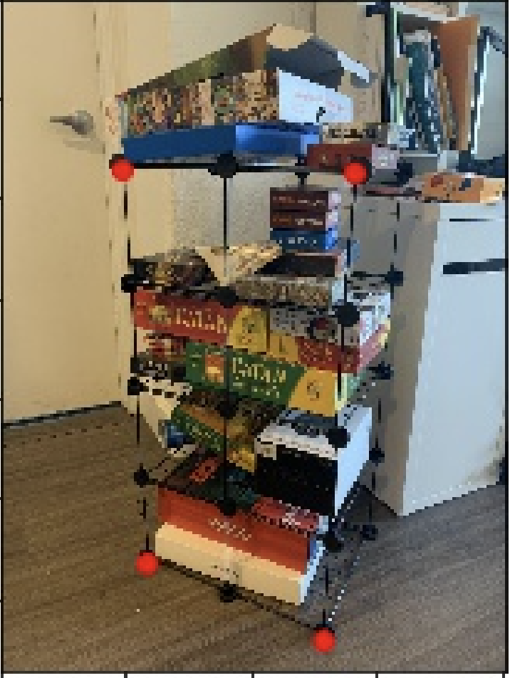 [250,0], [250,1000], [750, 1000], [750,0] |
 |
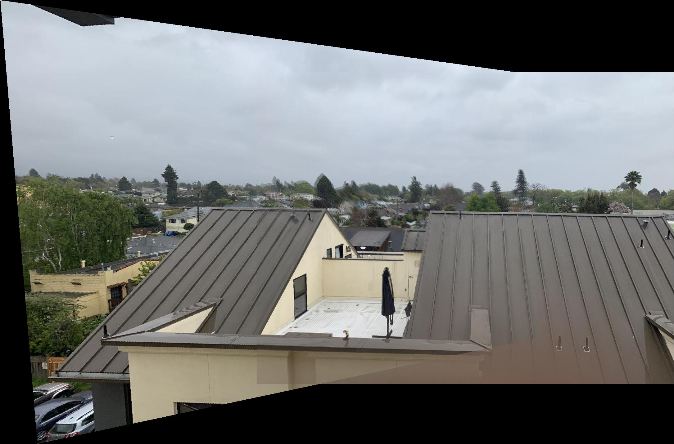
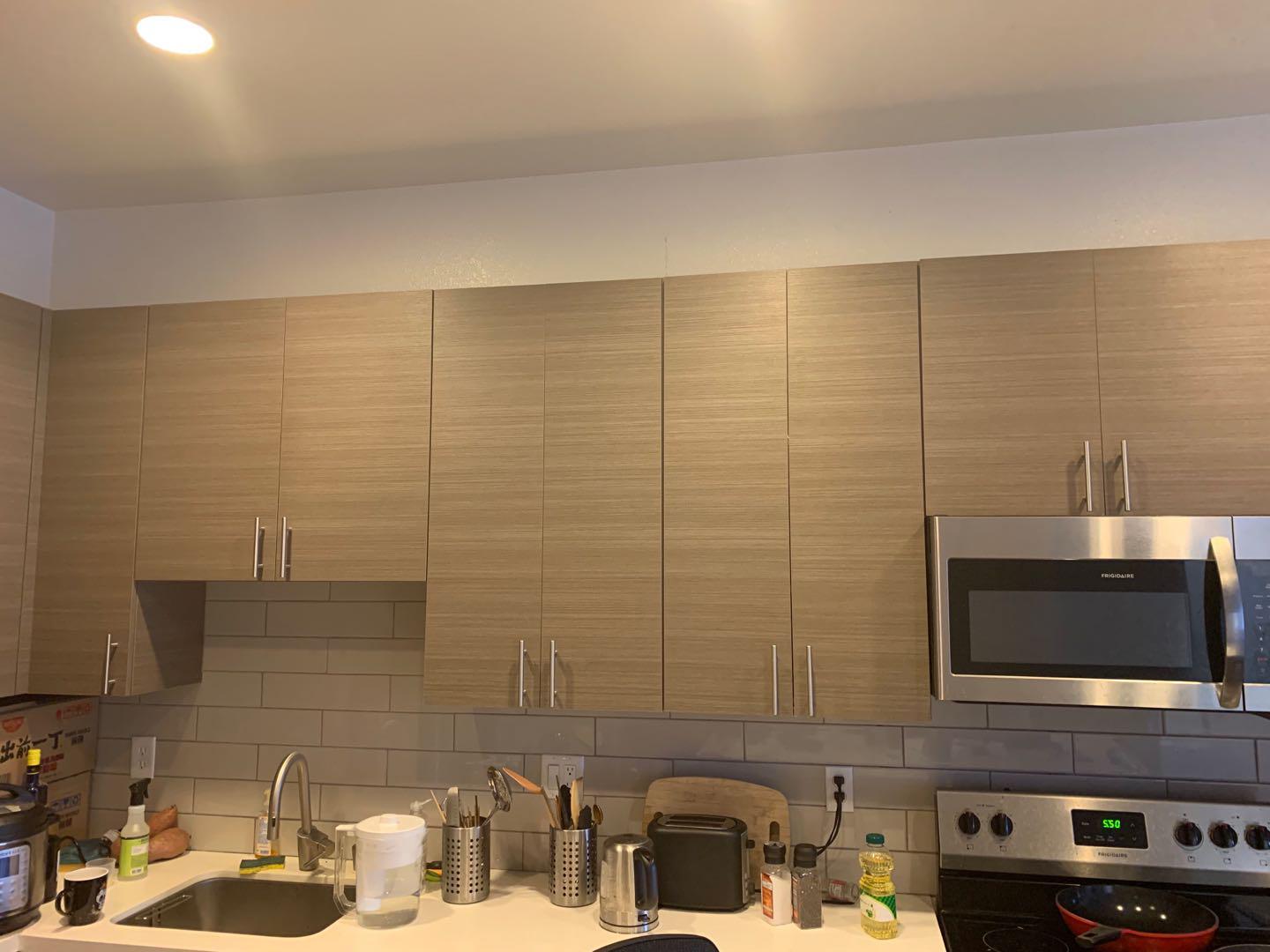
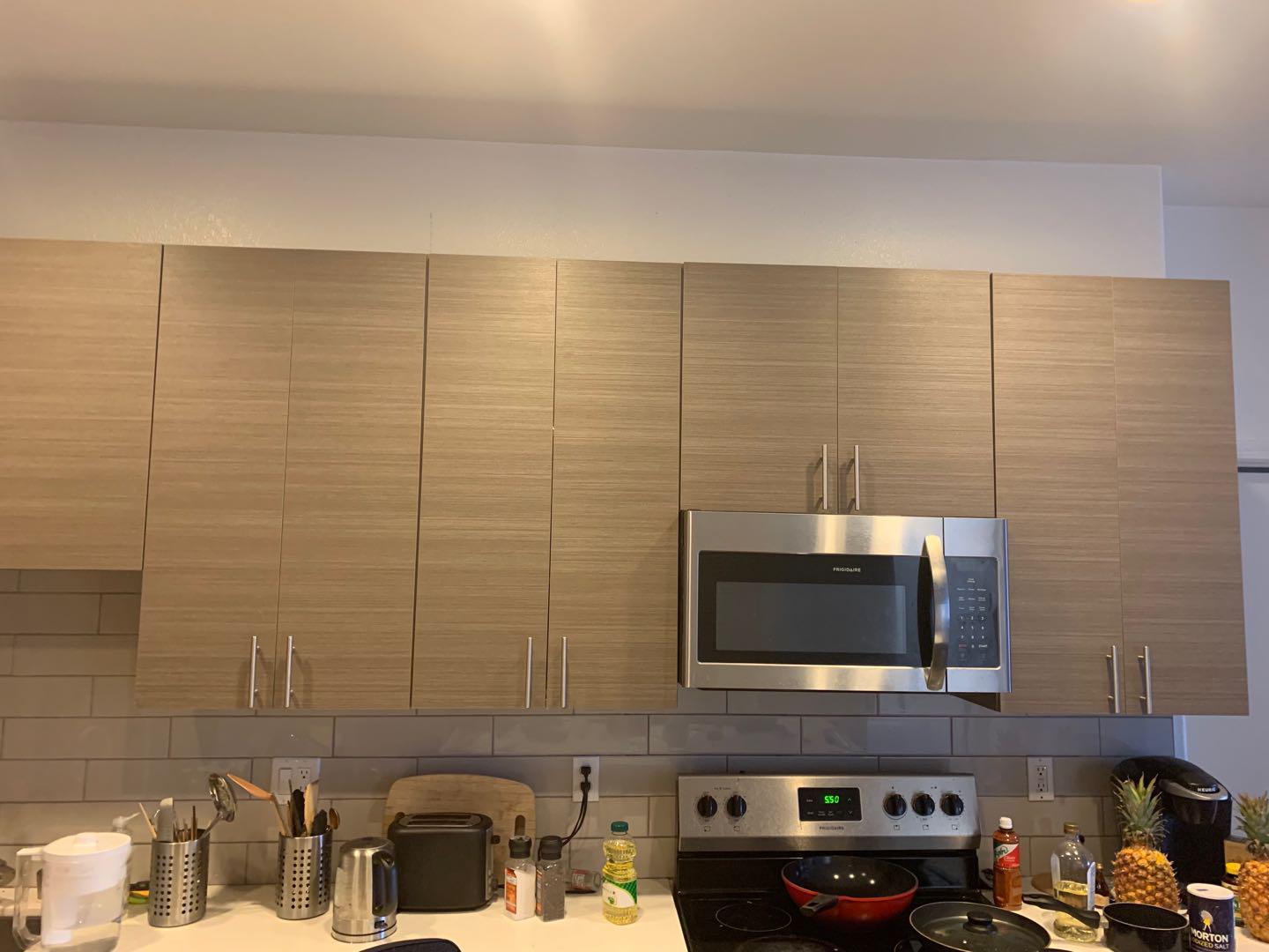
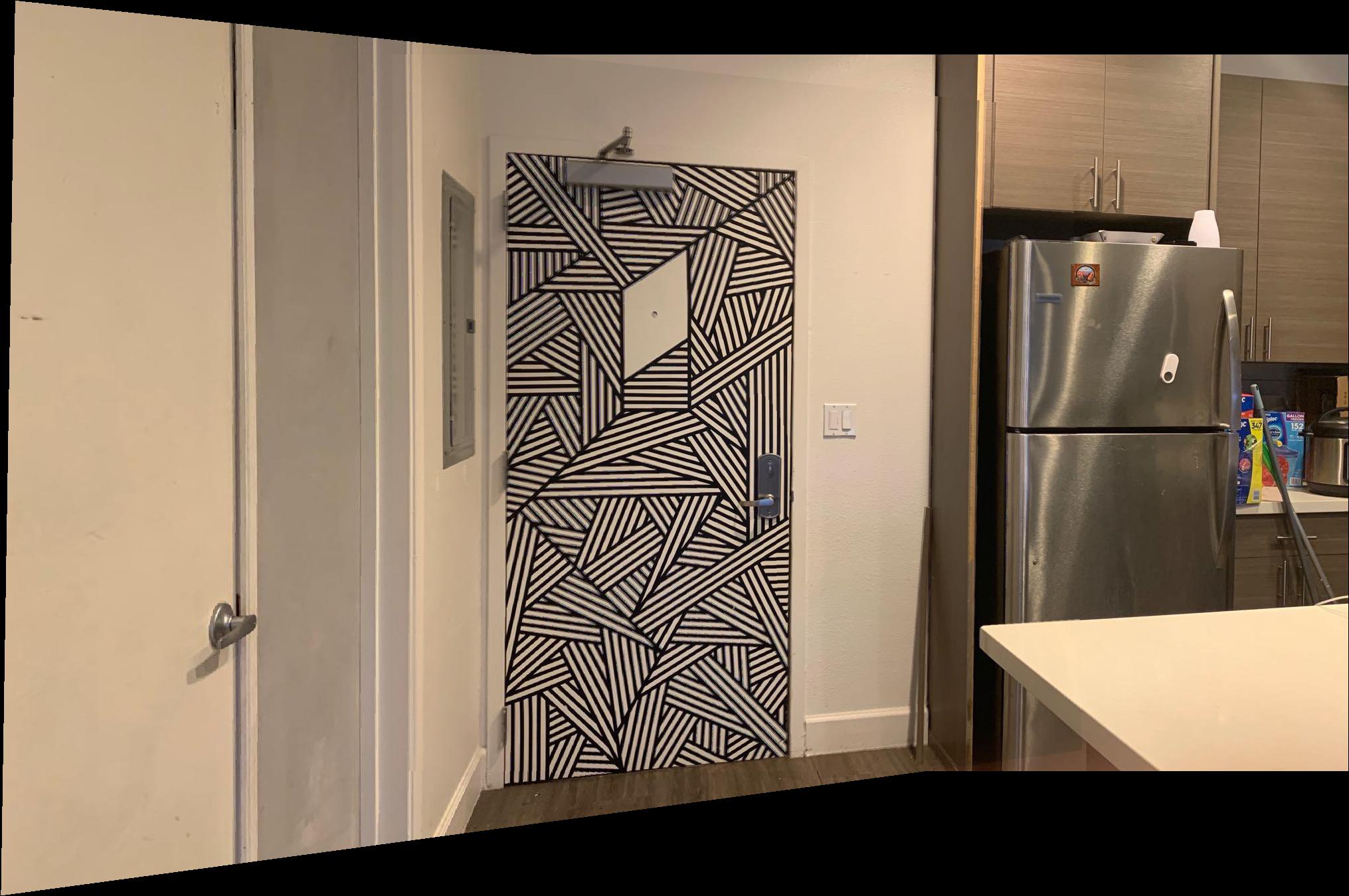
Similar to rectification, here I warped image 1 onto image 2 and put both images on a canvas that fits all pixels. For the overlapping area, I calculated the simple average of intensity from corresponding pixels in both images. Here are some examples,
| Image 1 | Image 2 | Mosaic |
|---|---|---|
|
|
 |
 |
 |
 |
 |
 |
 |
In this second part, we aim to replicate the above process without any manually labelled correspondence points. We will create a system for automatically stitching images into a mosaic. The algorithm is described by the paper Multi-Image Matching using Multi-Scale Oriented Patches
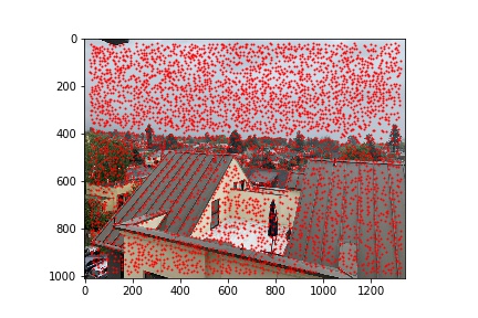
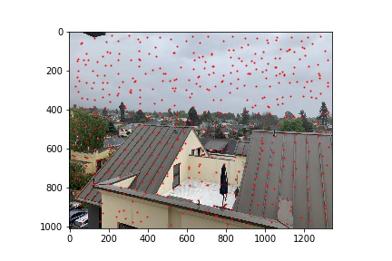
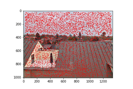
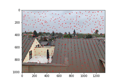
We begin by using the Harris Corner Detector to find all potential corners in our images. To get a fixed amount of interest points for an image and to have them as evenly spread out as possible, we implement Adapative Non-Maximal Suppression (ANMS) and set the target number of interest points as 500 and the robust buffer as 0.9. Here are the results.
| Original Image | Harris Point Detector | ANMS |
|---|---|---|
|
 |
 |
|
 |
 |
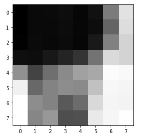
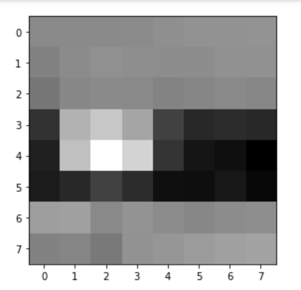
We then generate patches around each feature by first finding the 40 x 40 (41 x 41) square of pixels around each coordinate and then downsample the square to an 8 x 8 patch. Next, we calculate the SSD between all pairs of coordinates between both images. To reduce incorrect matches, we use Lowe’s outlier rejection algorithm, which only accepts point A from image 1 and point B from image 2 as a match if they are mutually the nearest neighbor (1NN) the other image and their SSD is some fraction of the average second nearest neighbor (2NN). We set the threshold to be 0.5 and the result is as follows.
| Original Image | Example Feature Patch | Matched Features |
|---|---|---|
|
 |
 |
|
 |
 |
With dozens of potential matching features in our hand, we now need a way to distinguish good matches from bad matches and produce a homography from the subset of good matches. Using RANSAC, we produce a homography based on 4 randomly chosen pairs from all features points and calculate the Euclidian distance between every projected feature point and their correspondence. I set ssd = 1 as the cutoff; therefore, all feature pairs with less than 1 unit of difference will be considered inliers. Iterating the above process for 100000 times, and compute a homograph based on the largest set of inliers will give us the result of auto-stitching. Here is the comparison of results from manually labelled feature points and the above auto-stitching process.
| Image 1 | Image 2 | Manually stitched | Auto-stitched |
|---|---|---|---|
|
|
|
 |
|
|
|
 |
|
|
|
 |
As you can see, the results are very almost idential to the manually labelled images. This shows that our implementation works correctly and is in part because I manually labelled around 30 points in Part a to avoid any errors.