Project Overview
In part A of the project, we apply perspective transforms on images for rectification and for creating panoramas.
Part 1: Image Rectification
The first thing we need to do if to define some correspondences. For image rectification, we can find a planar shape in the original photo, and then define some points that we would like them to be transformed to. For example, in the following photo that I took at Bay Street, Emeryville, I marked the four corners of one painting and then define their correspondences into a frontal-parallel square shape. Then, we compute the homography (represented by a 3x3 matrix, 8 degrees of freedom) between the two set of points by performing least-squares on the correspondence points to find the coefficients in the homography matrix H. The formula is as follows.
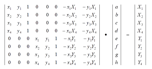 Image from Google
|
After finding H, I used inverse warping to create the rectified images. Because the transformed images can no longer fit into the same dimensions, I created a new bounding box based on where the four corners of the original image is mapped to according to H. Here are some rectified results.
 Photo of a little swan maded out of snow (yes, the beak is a piece of orange peel...)
|
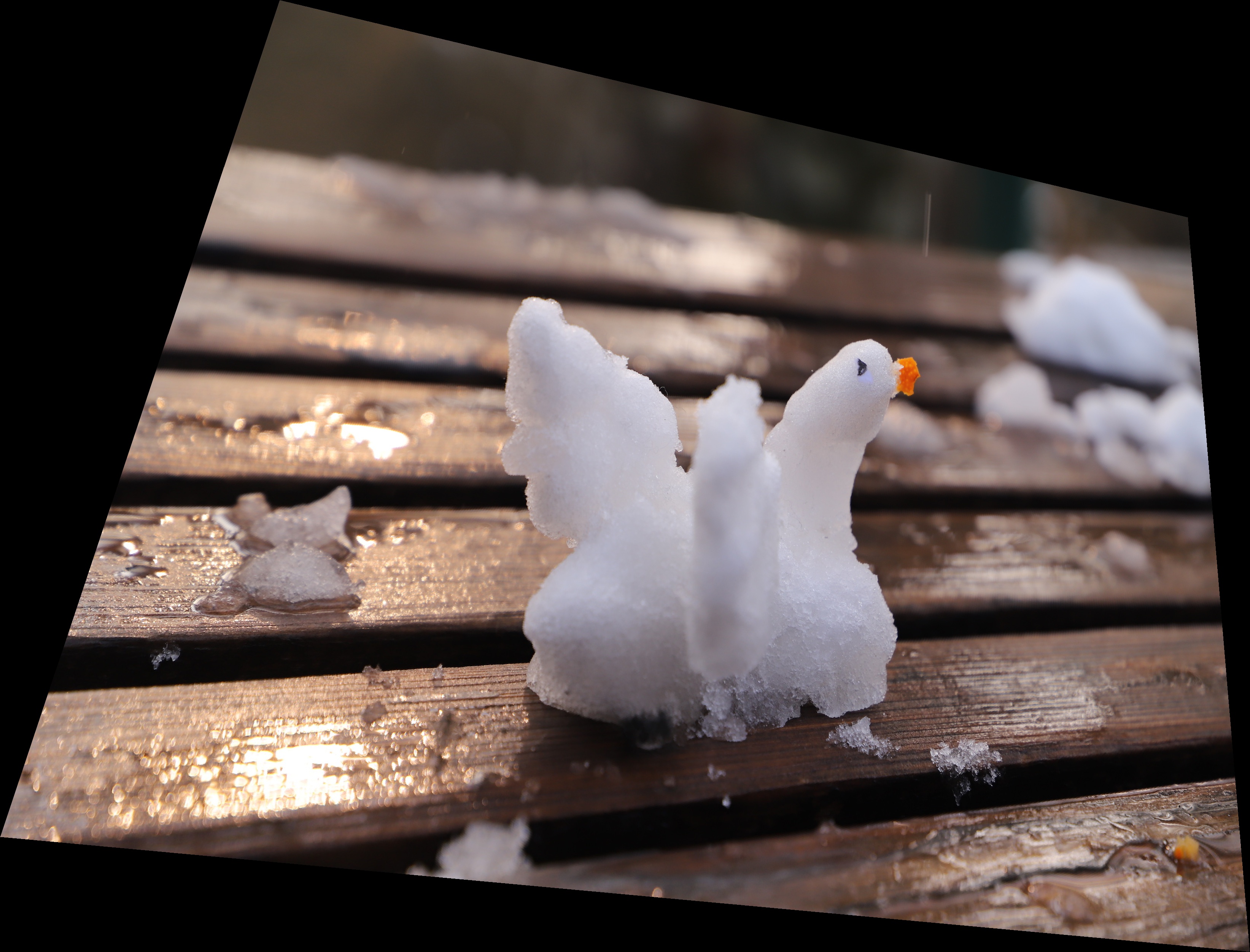 Warped Swan
|
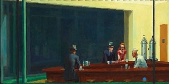
I also tried to rectify this famous painting Nighthawks by Edward Hopper. I warped the painting so that the view into the window of the bar is frontal-parallel. Interestingly, after the perspective is changed, the gloomy vibe and the portrayal of lonely urban life seems much less pronounced. Perspective really shapes the artistic mood!
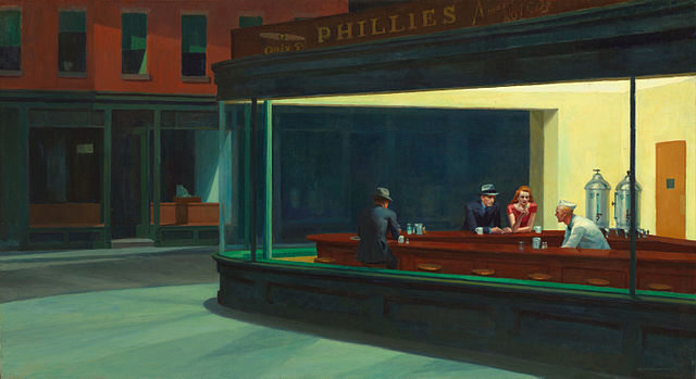 Nighthawks by Edward Hopper
|
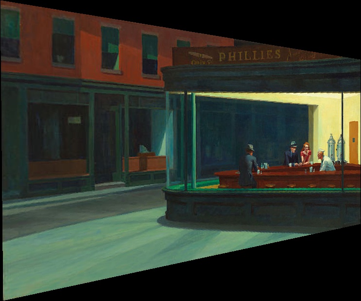 Warped Nighthawks
|
 Warped and cropped Nighthawks
|
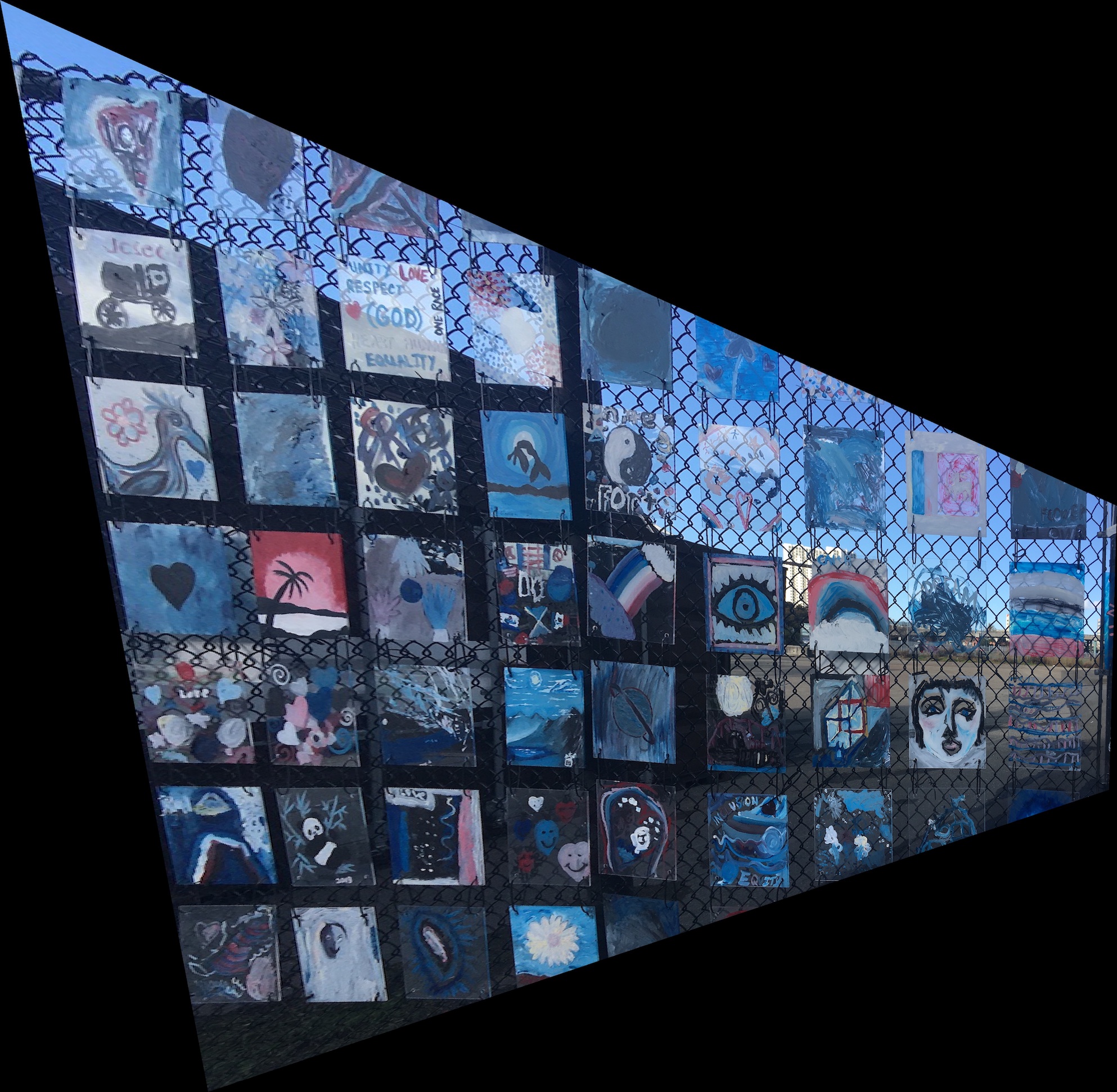
Finally, I rectified this photo I took at Bay Stree, Emeryville. It was a wall of paintings, and I'd argue some of them can compete with the nighthawks! I rectified this photo to force the one of the paintings (the one that has a face) into a square shape. Here are the results.
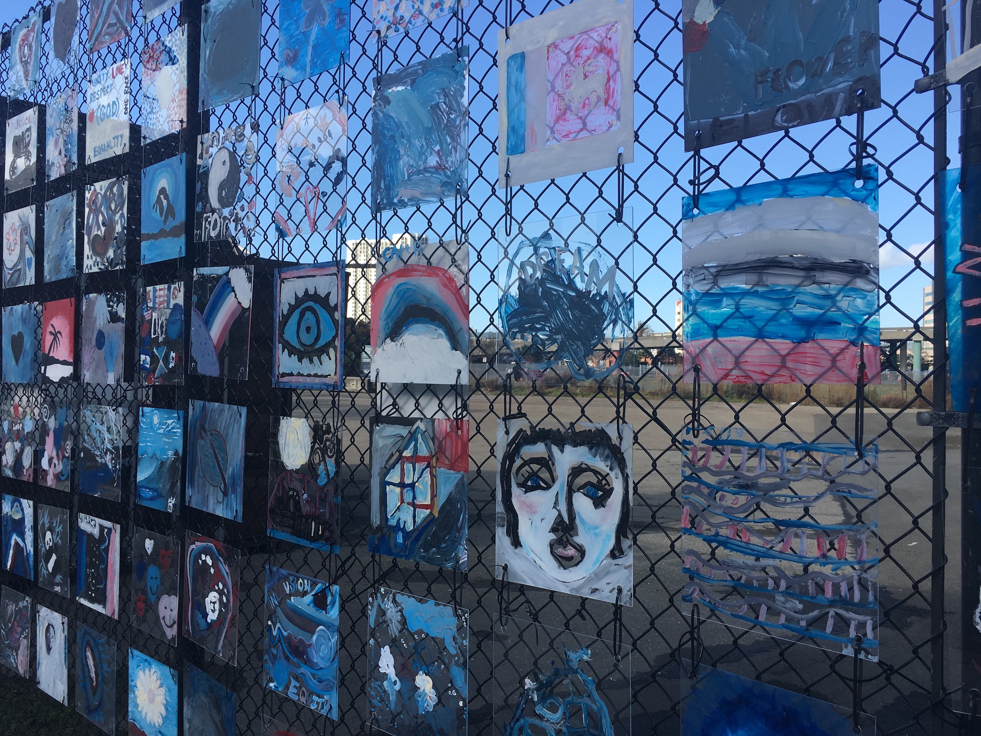 Painting Wall at Emeryville
|
 Warped
|
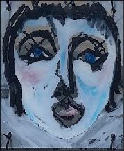 Warped and zoomed in (great painting indeed!)
|
Part 2: Image Mosaic
In this part, we stitch together two images. First, we rectify the first image to the perspective of the second image. Then, with an alpha mask, we blend the warped first image and the original second image together to form a bigger mosaic.
Here are some results!
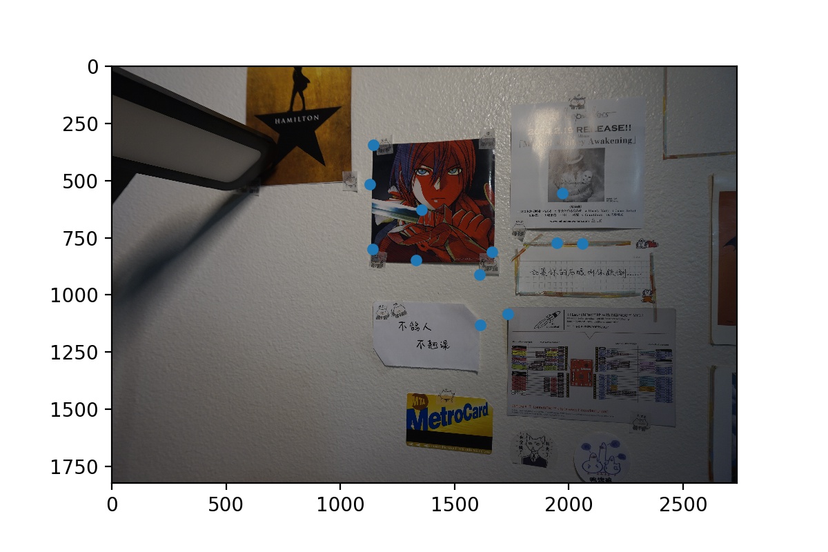
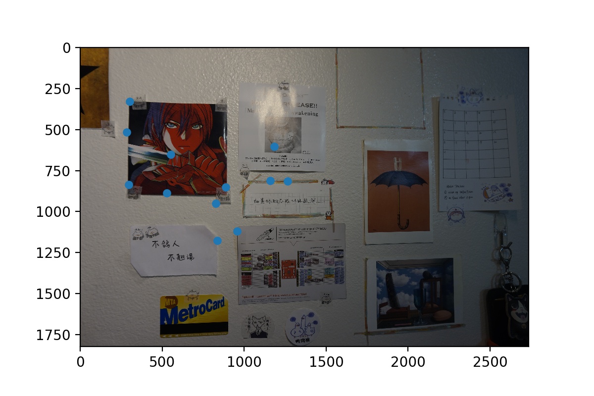
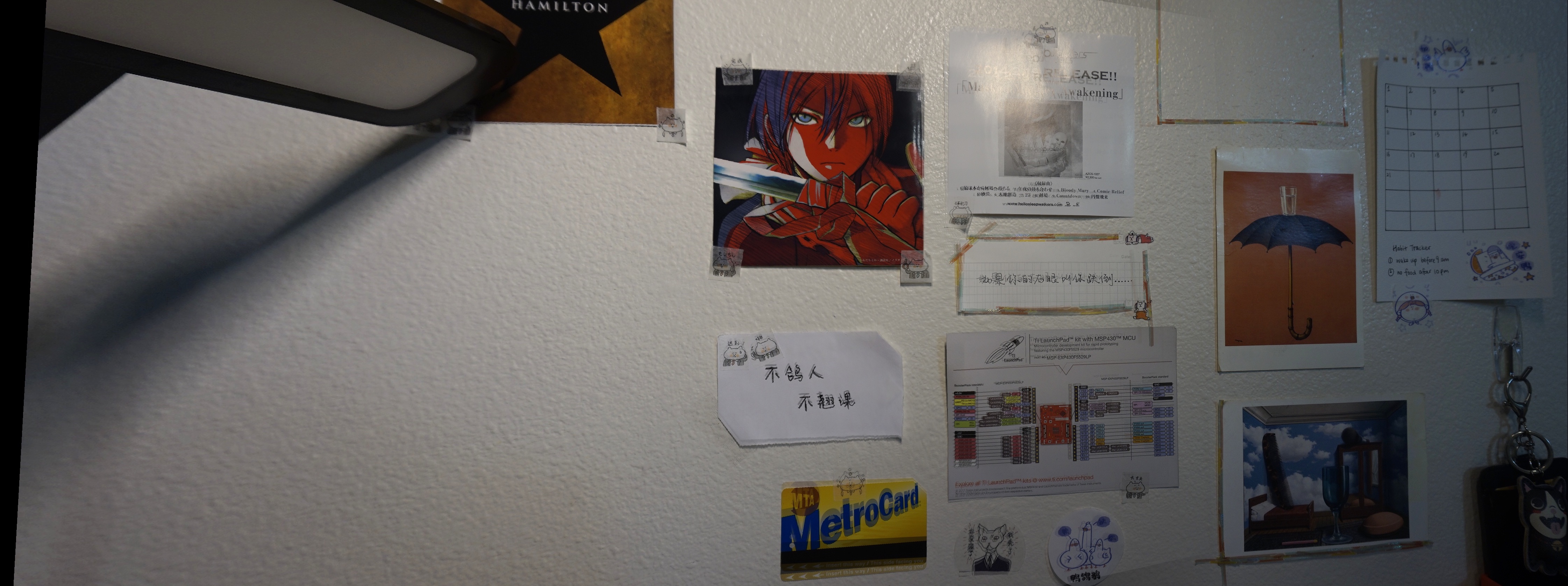
This is a mosaic of the wall in front of my desk in my room. I decorated it with lots of mementos and postcards. (Right in the center is a pin manual for the launchpad(s) I used in EE16B. I put it there to remind myself that if I could overcome the sweet struggle of mysterious hardware failures, then I can overcome anything in the world lol)
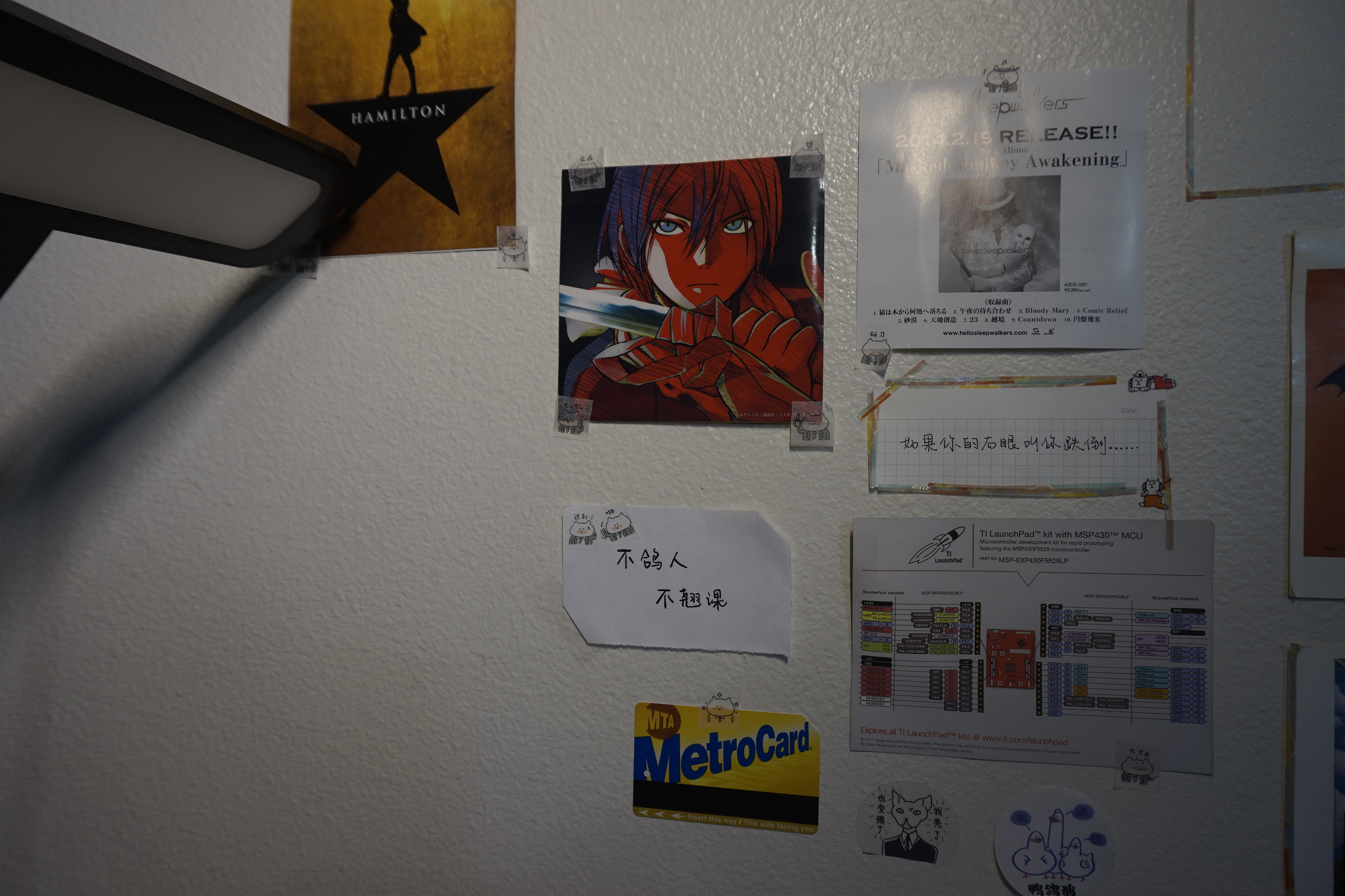 Image 1
|
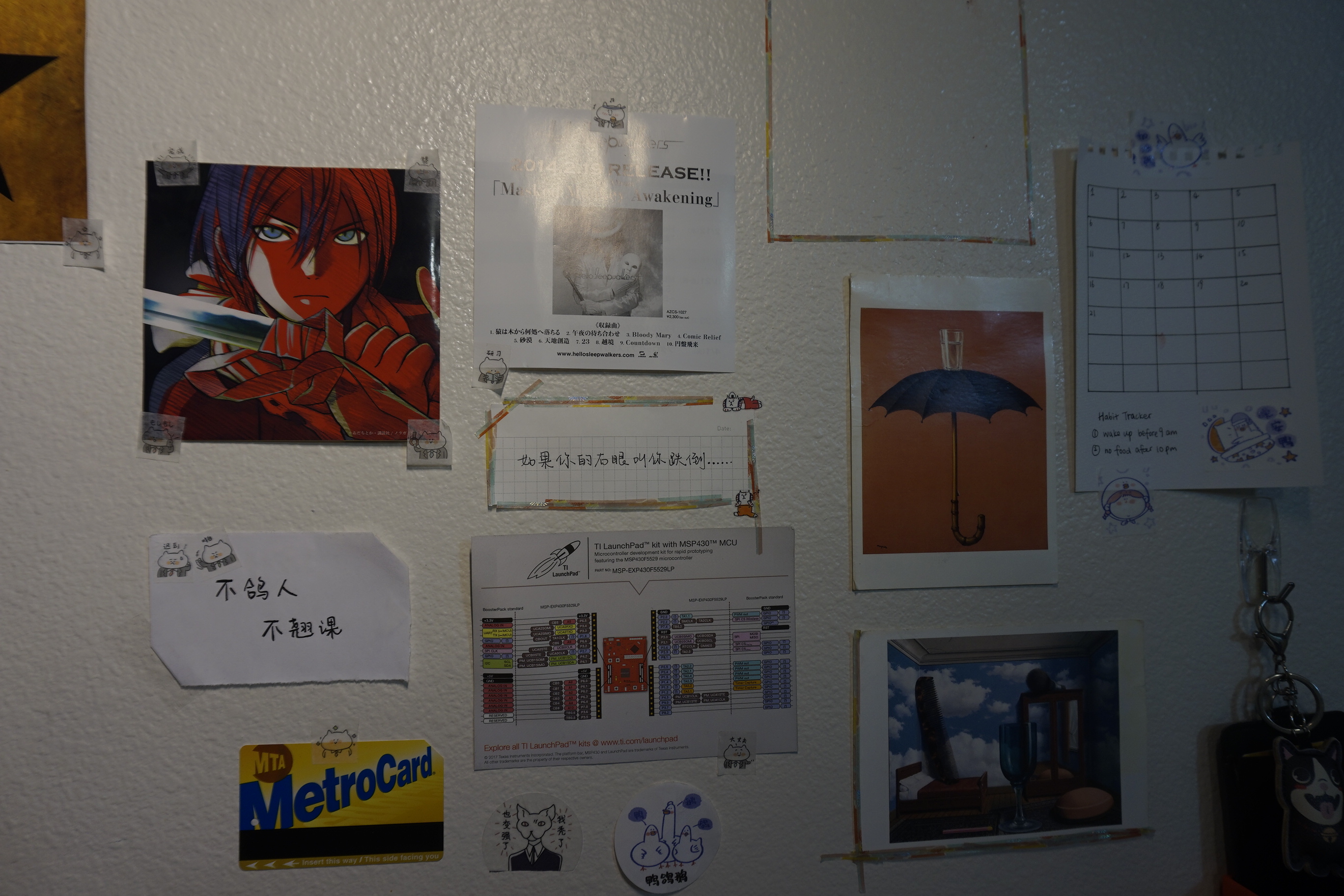 Image 2
|
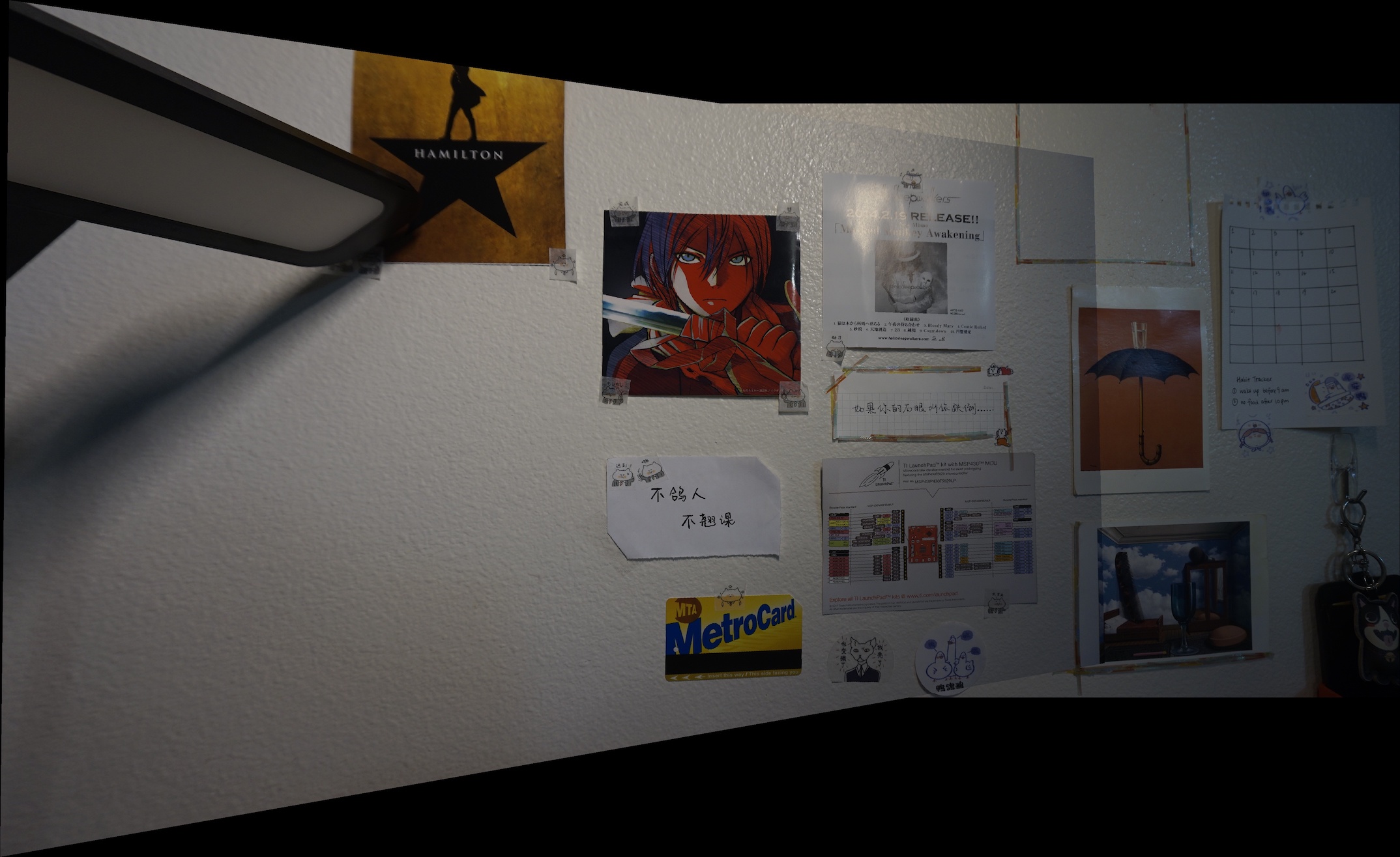 Mosaic with direct blending
|
We can see that there are some edge artifacts around the borders of the overlap region between the two images, so I used feathered alphablending to smooth out these borders.
 Feathered Mask
|
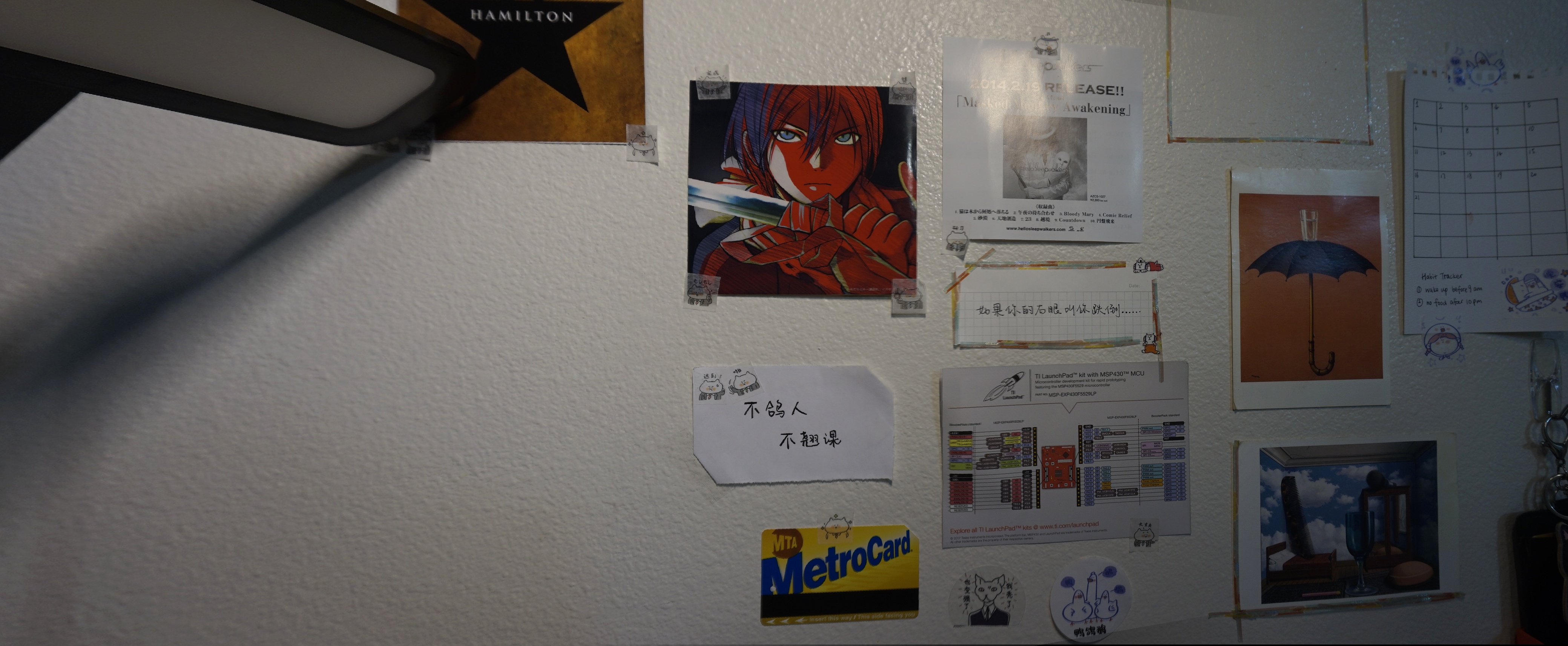 Mosaic with alpha blending (cropped)
|
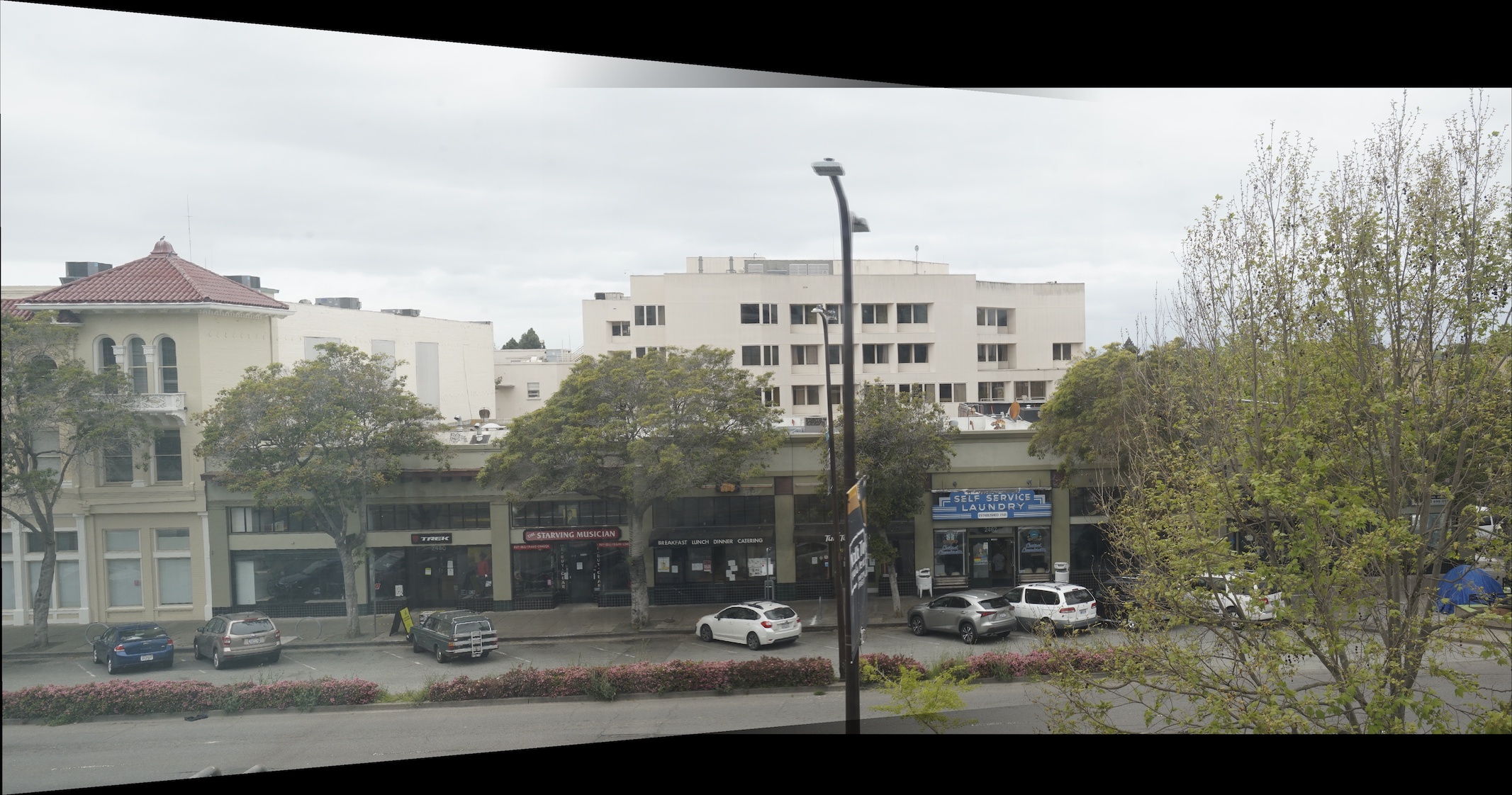
Here are some more results of outdoor scenes.
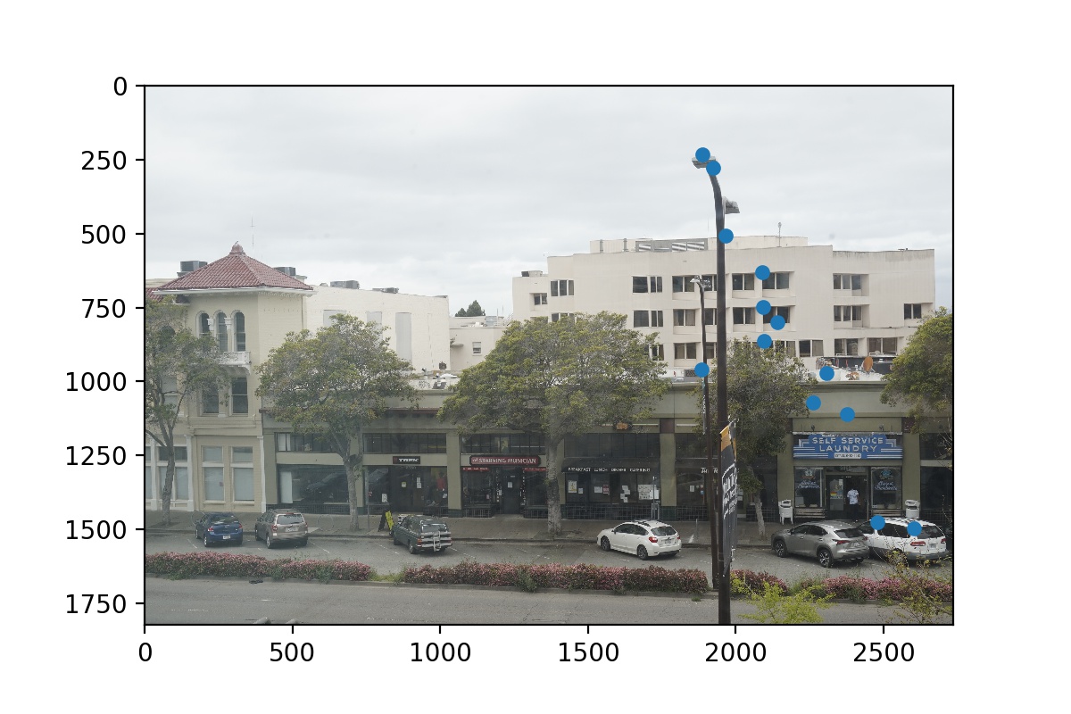
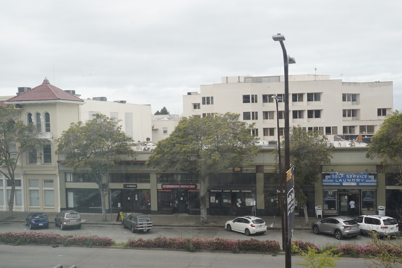 Street View 1
|
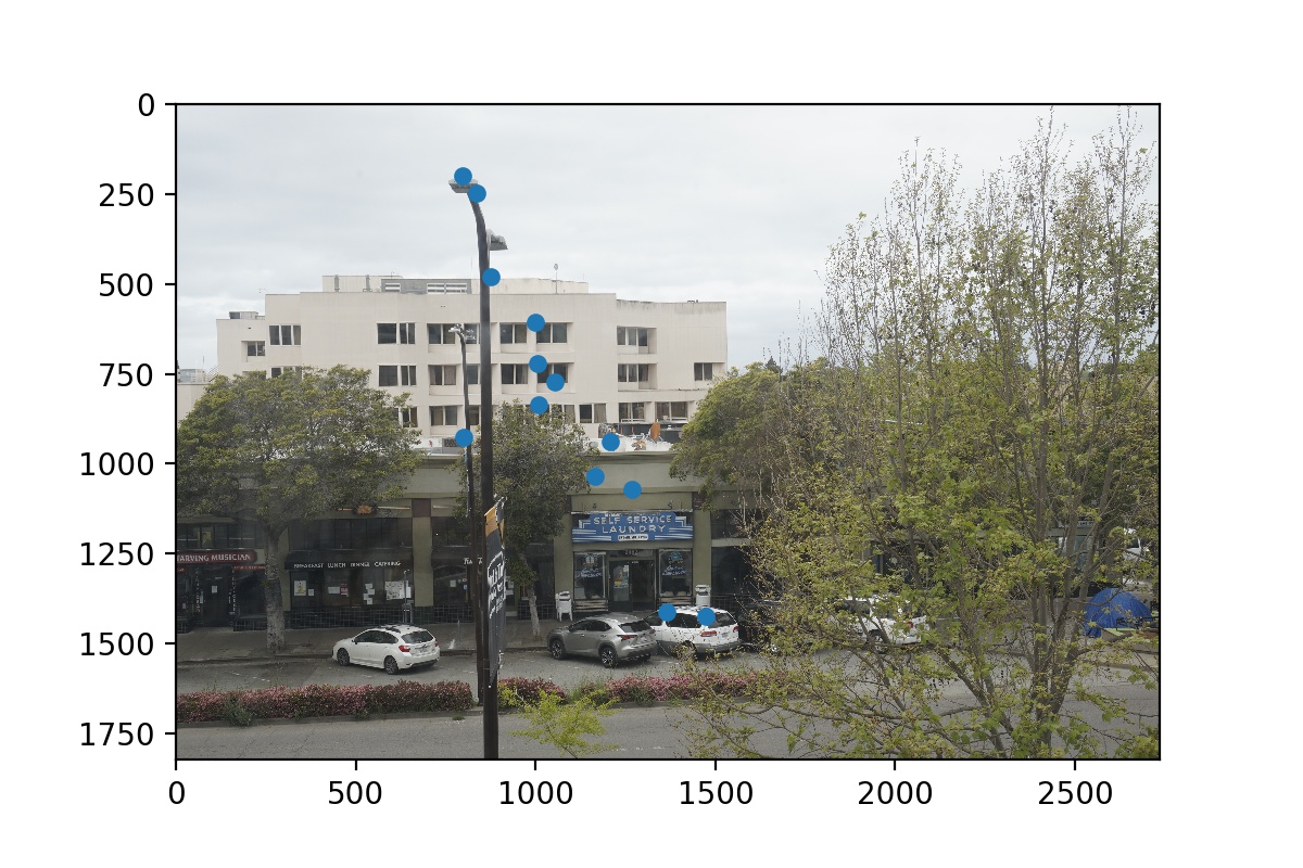
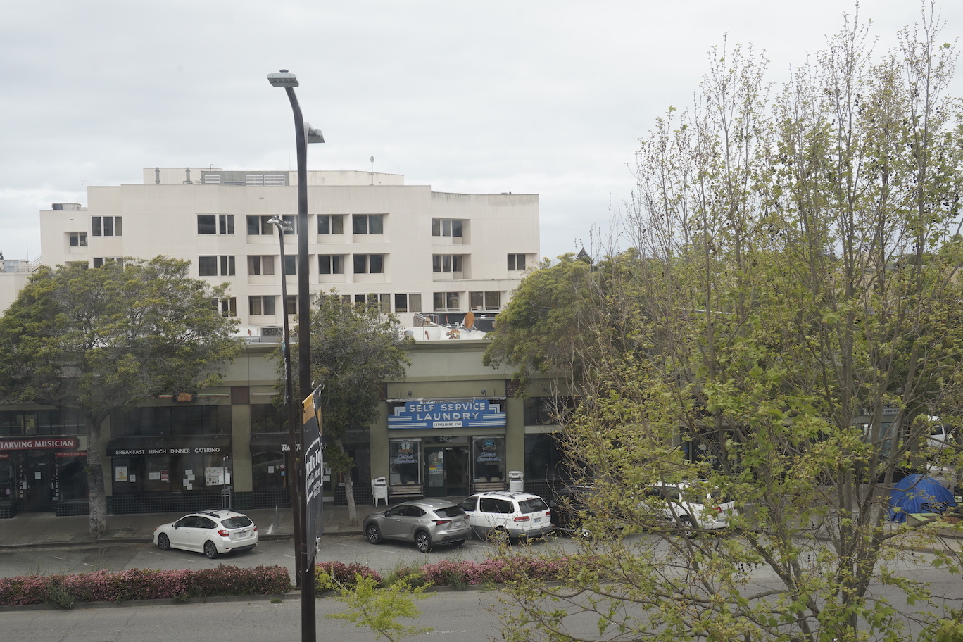 Street View 2
|
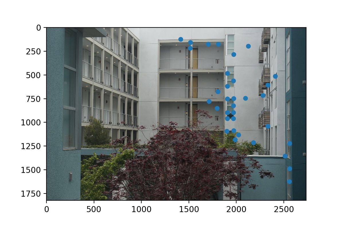
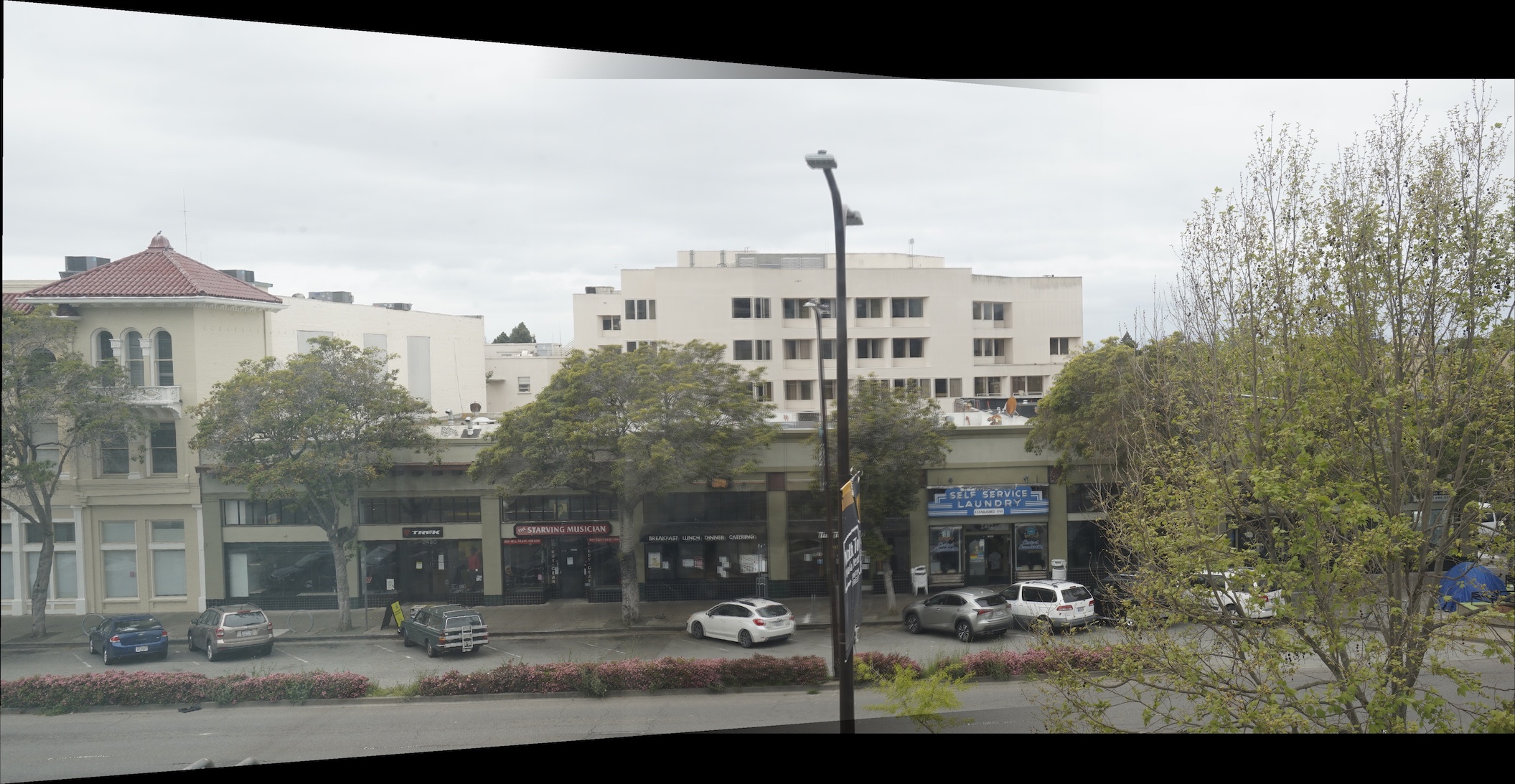 Street View Mosaic
|
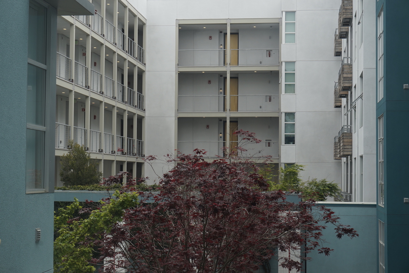 Image 1
|
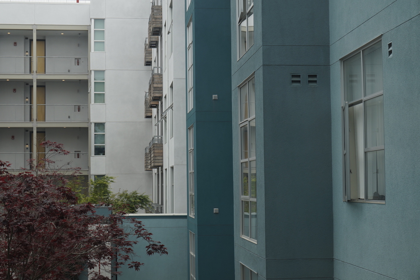 Image 2
|
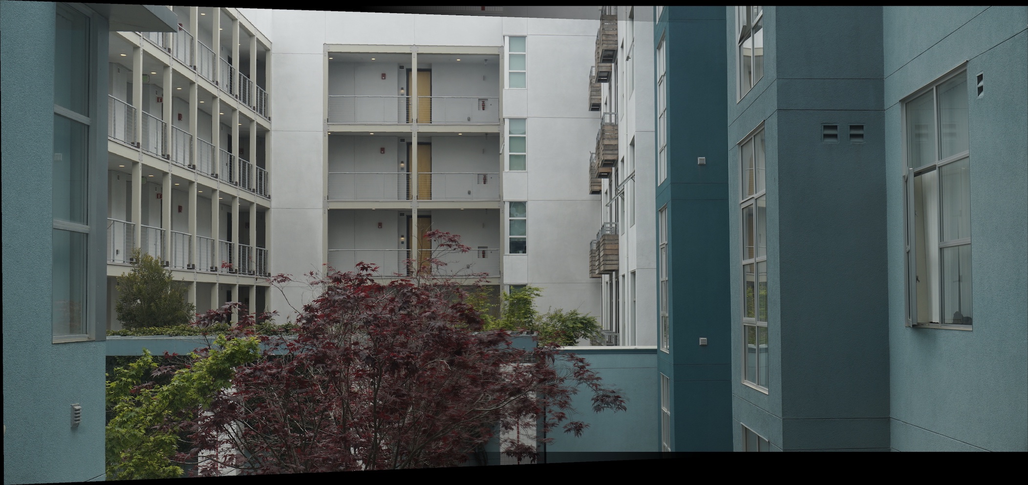
 Courtyard Mosaic
|
Part 3: Auto-Stitching with Feature Matching
Manually defining correspondence points is very draining, so we implemented this automatic procedure to find matching interest points across two images. The following procedure is adapted from the paper “Multi-Image Matching using Multi-Scale Oriented Patches” by Brown et al."
Step 1: Finding Harris Corners
First, for each image in the mosaic, we need to perform feature extraction. We do this by first finding harris corners within the mosaic.
 Harris Corners of Wall View 1
|
 Harris Corners of Wall View 2
|
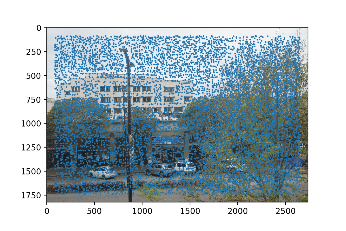
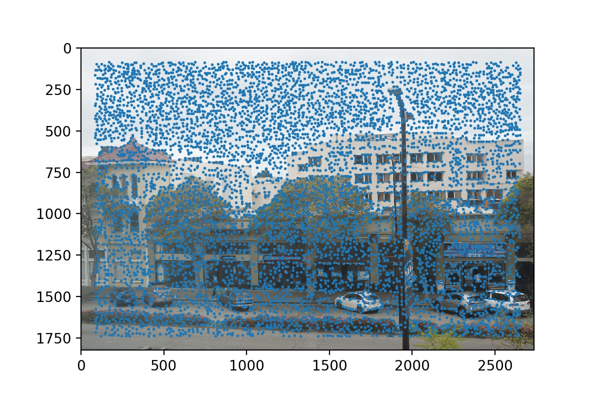 Harris Corners of Street View 1
|
 Harris Corners of Street View 2
|
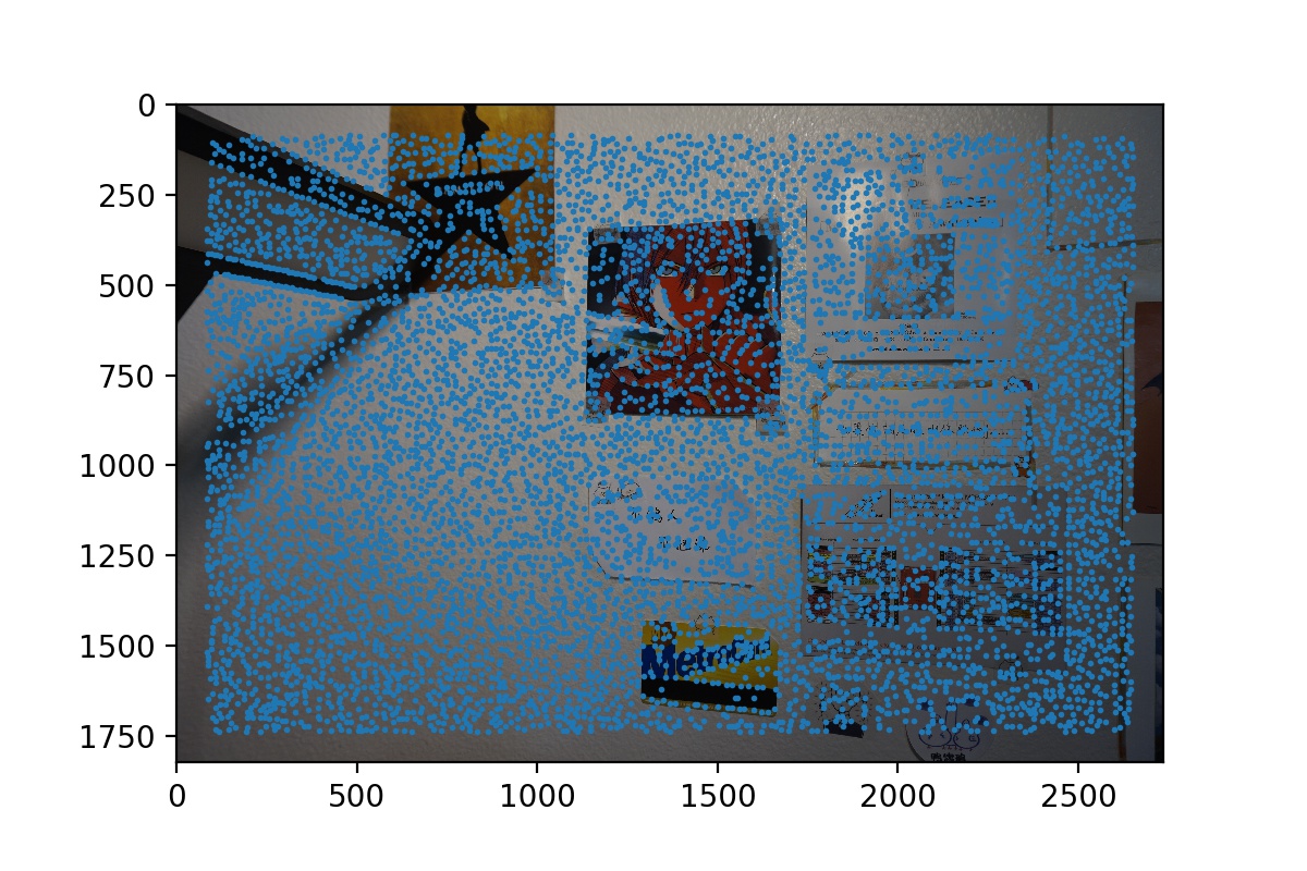
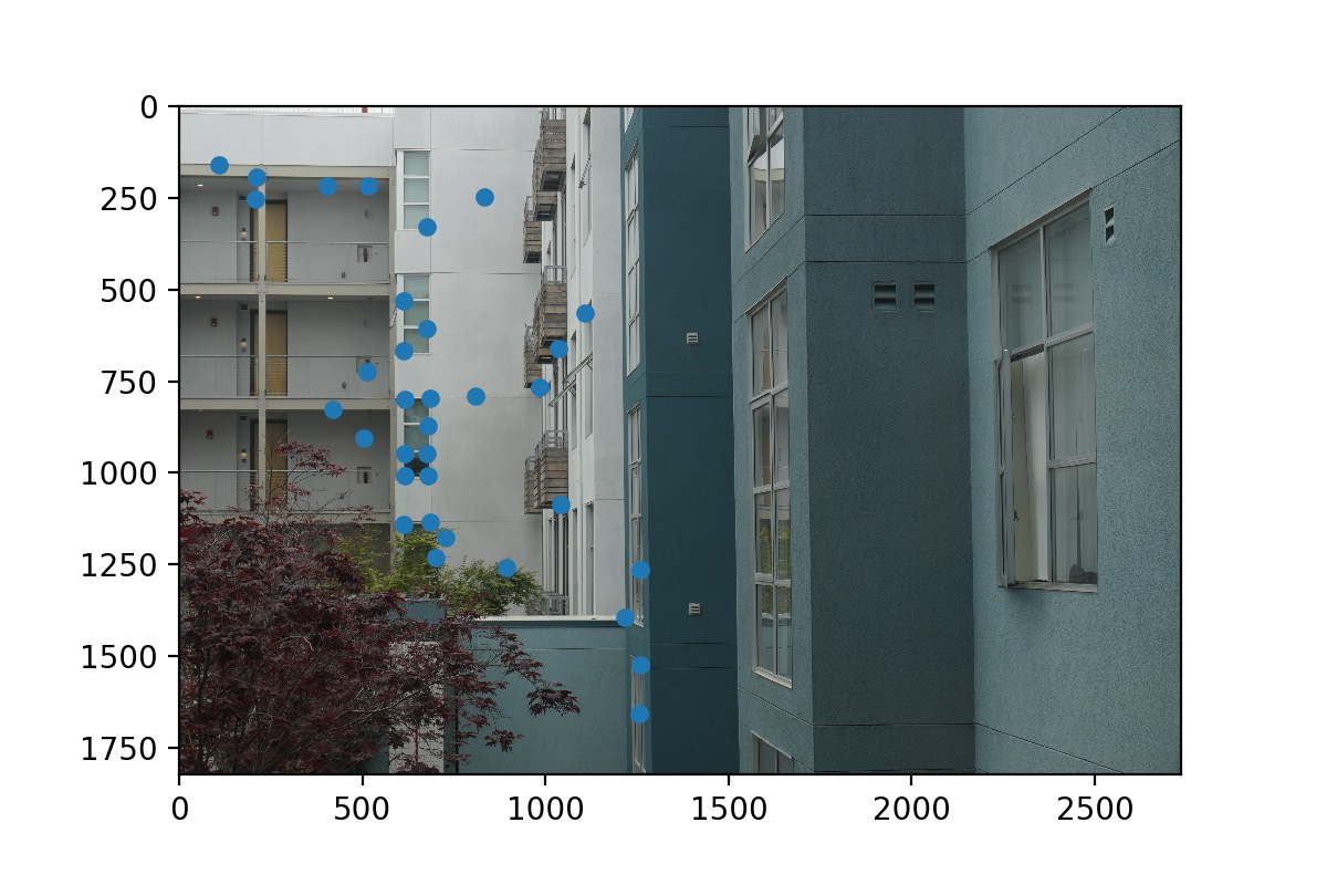
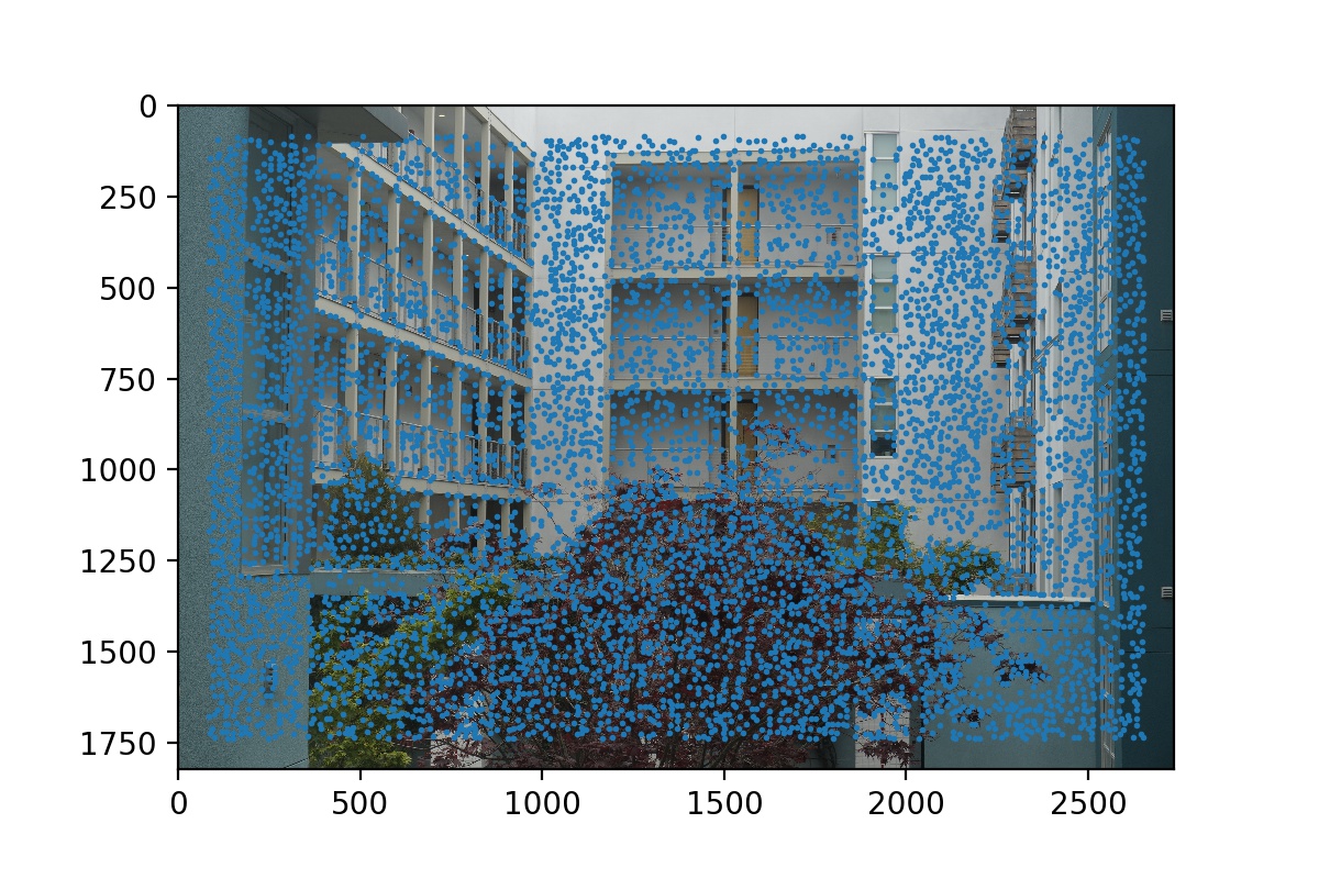 Harris Corners on Courtyard View 1
|
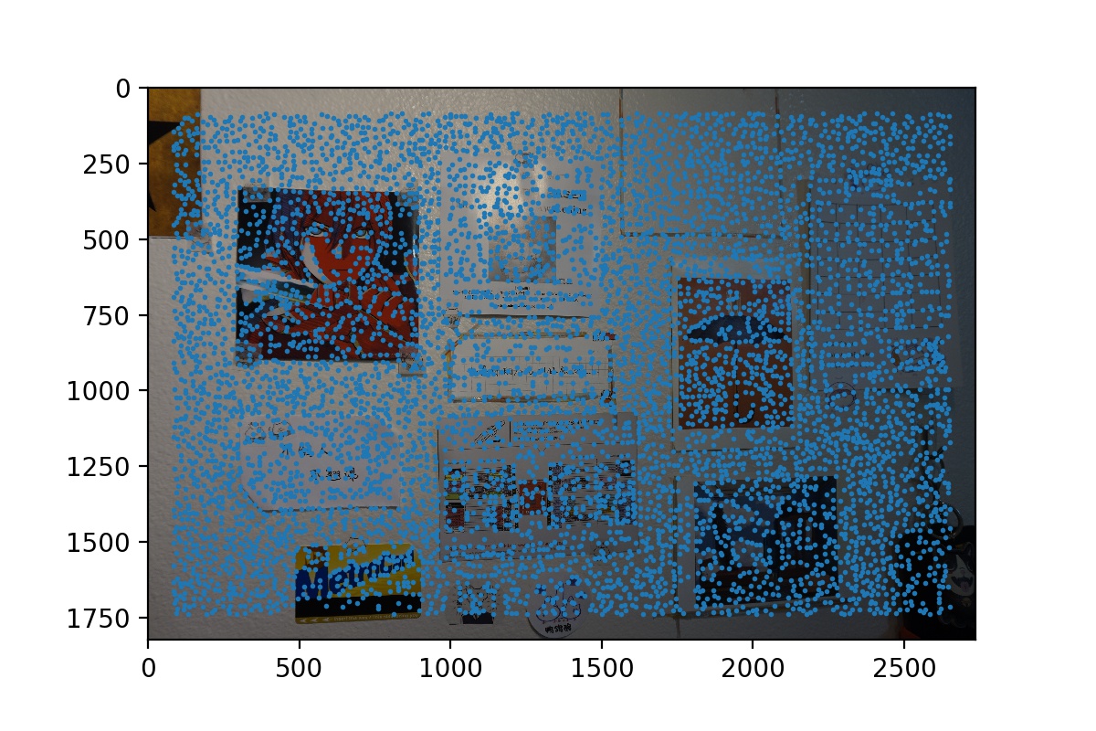
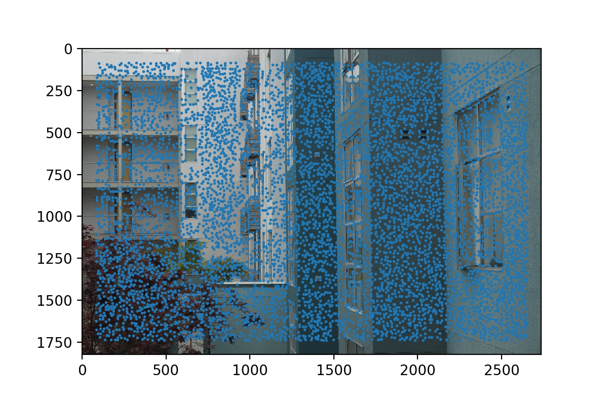 Harris Corners on Courtyard View 2
|
Step 2: Adaptive Non-Maximal Suppression
We select the 500 most promising corners using Adaptive Non-Maximal Suppression. We basically compute a suppression radius for each corner and select the top 500 corners with the highest suppression radius. The suppression radius of a corner is computed by its minimum distance to any other corner that has a higher corner strength. In this way, we make sure that the selected corners are most likely representing distinct and well-distributed features in the image.
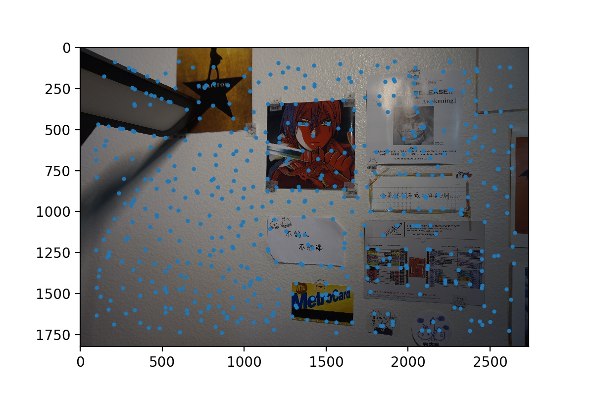 Post-ANMS Corners of Wall View 1
|
 Post-ANMS Corners of Wall View 2
|
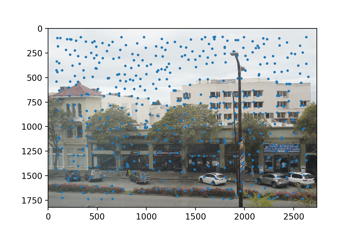 Post-ANMS Corners of Street View 1
|
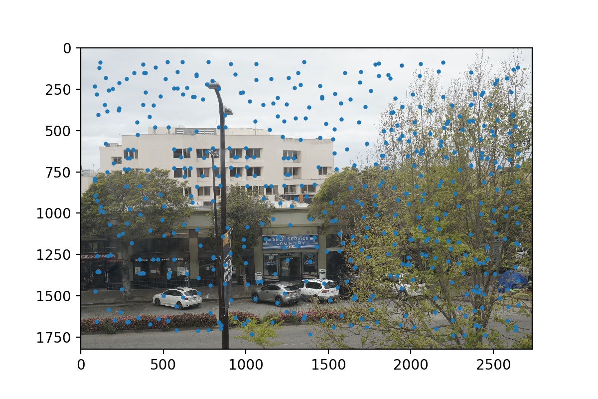 Post-ANMS Corners of Street View 2
|
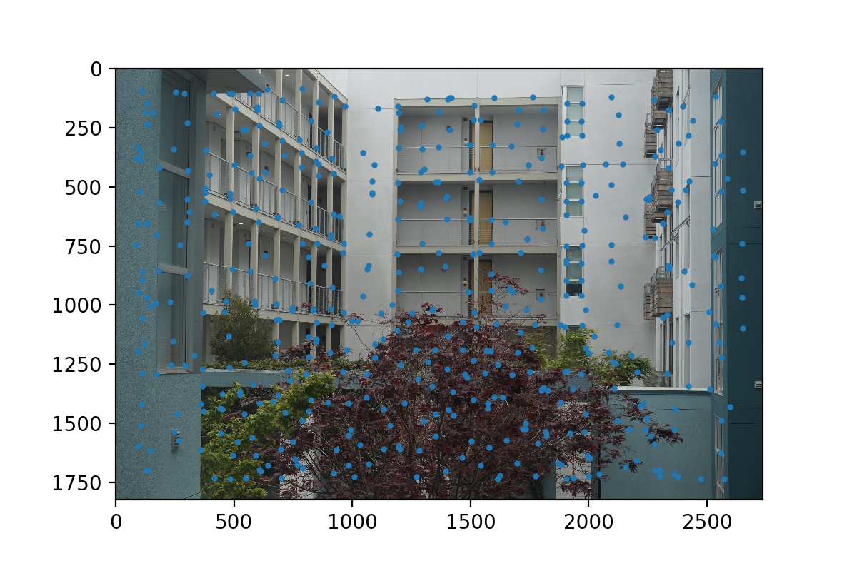 Post-ANMS Corners of Courtyard View 1
|
 Post-ANMS Corners of Courtyard View 2
|
Step 3: Generate Feature Descriptors
After finding the 500 interest points, we describe each of them using a 8x8 vector descriptor. We take the 40x40 neighborhood patch of each interest point and subsample it with a scale of 5. Then, we normalize the 8x8 vector so that it has mean = 0 and standard deviation = 1 so that our feature matching will not be influenced by bias.
Step 4: Match Feature Descriptors with 1NN/2NN Ratio Thresholding
After we obtain a list of 8x8 vector descriptors of the feature points in each image in the mosaic, we can now match them. We use Lowe’s procedure to filter out correct matches. For each feature in image A, we compare its descriptor to all the feature descriptors in image B using SSD. We find the closest and second closest feature in B to the feature in A, and we compute the ratio of their SSD error. If this ratios is smaller than the threshold (=0.3), then we take this pair to be a possibly correct feature matching. If the ratio is higher, we reject this pair. This algorithm is based on the fact that if a pairing is correct, then it should have significantly less error than whatever is second closest to correct but definitely wrong, since there can only be one true correct corresponding feature in B that matches to the feature in A.
Step 5: RANSAC
After this filtering process, we may still be left with many wrong matches, so we run RANSAC to further distinguish correct matchings and incorrect matchings. We randomly choose four pairs of matchings, and compute a homography based on them. Then, we count how many inliers we would have given this homography transformation. After doing so for 10000 iterations, we keep the largest set of inliers we have found and compute a least-squares homography based on these inliers. The result would be the final homography that we have found to warp the image!
 Post-RANSAC Features of Wall View 1
|
 Post-RANSAC Features of Wall View 2
|
 Post-RANSAC Features of Street View 1
|
 Post-RANSAC Features of Street View 2
|
 Post-RANSAC Features of Courtyard View 1
|
 Post-RANSAC Features of Courtyard View 2
|
Step 6: Warp Image and Create Mosaic
After obtaining this homography, the rest of the mosaicing is the same as part 2. We warp the first image and then blend it with the second image to form a larger mosaic.
Auto-stitching Results
Let’s compare the mosaic results using manual vs. automatic homography finding. We see that they are very similar. Up close, the manuel mosaic of the street view is a bit more blurry than the auto-stitched because my manually selected correspondence points may be a bit inaccurate, and also I only selected ~10 points for that set of images manually. The other two sets mosaics look almost identical.
|
Manual Mosaic
|
 Wall Auto-stitched Mosaic
|
|
Manual Mosaic
|
 Street Auto-stitched Mosaic
|
|
Manual Mosaic
|
 Courtyard Auto-stitched Mosaic
|
Final Reflections
This project has been really fun. It’s really amazing to be able to find homographies automatically using these data-driven methods and filtering procedures. The Adaptive Non-Maximal Suppression, 1NN/2NN ratio thresholding, and RANSAC procedures are intuitively meaningful and practically effective. I learned a lot through implementing them, and I really wish that I could have gone outside to take better photos for cooler panoramas!