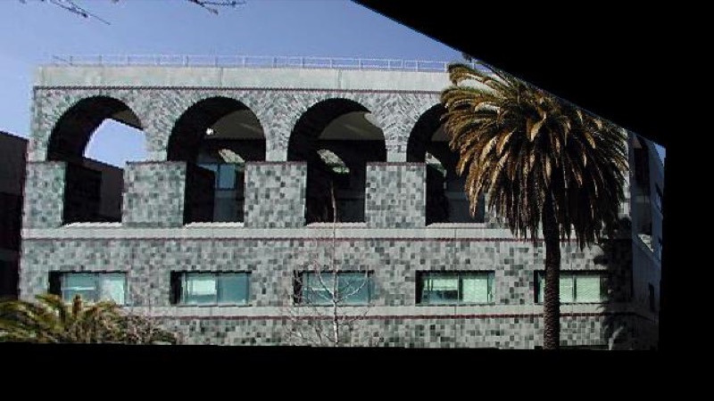
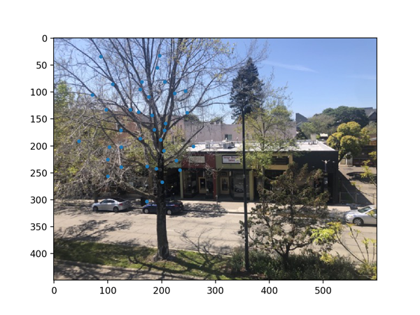
Here are the two pictures that I shoot for image rectification
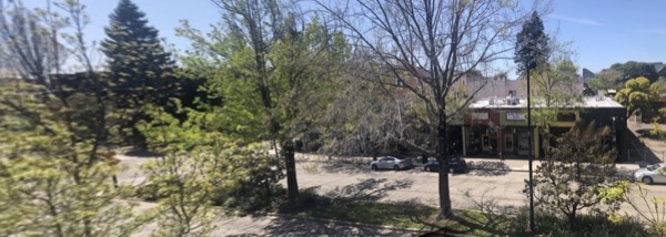
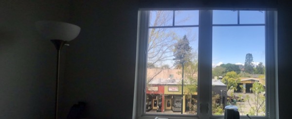
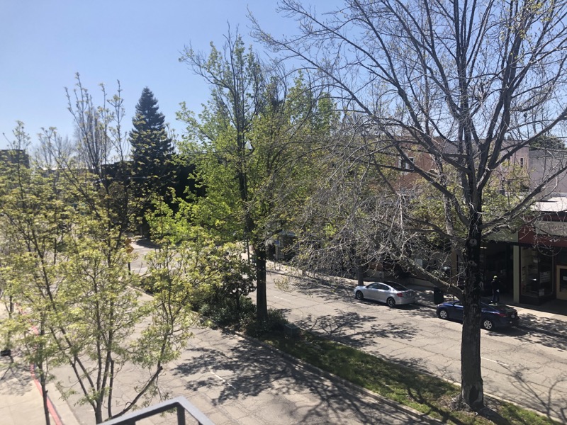
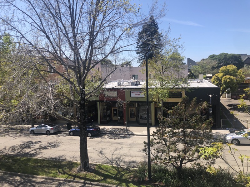
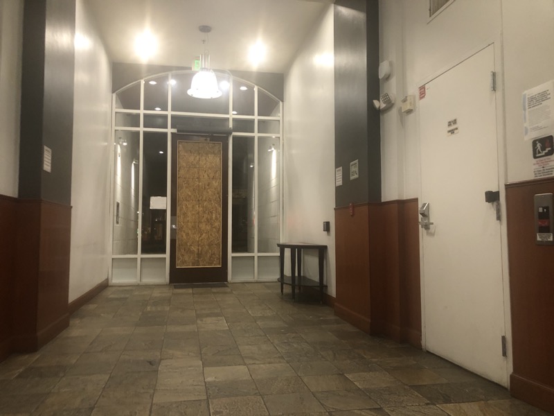
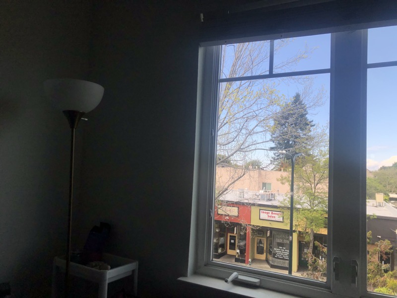
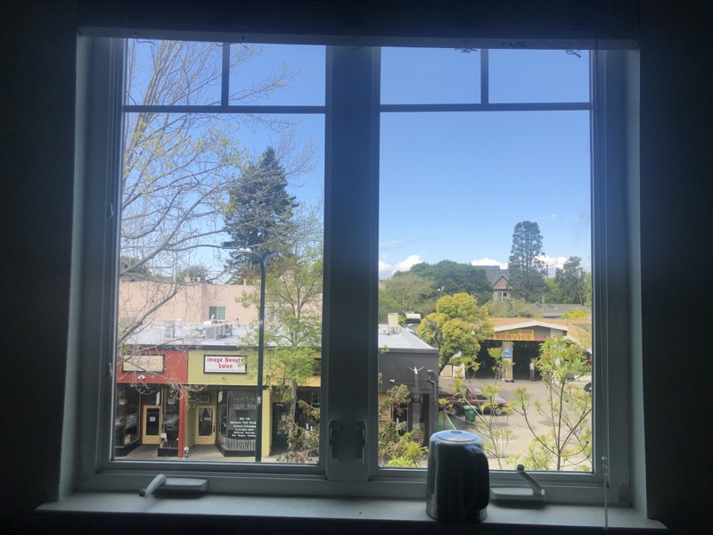
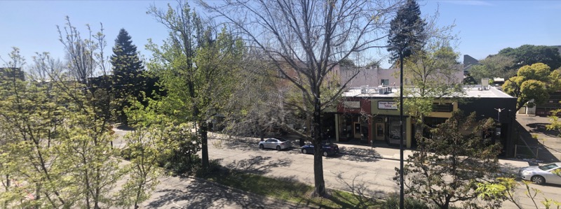
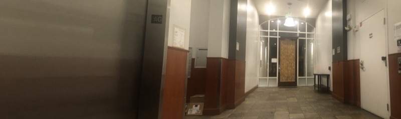
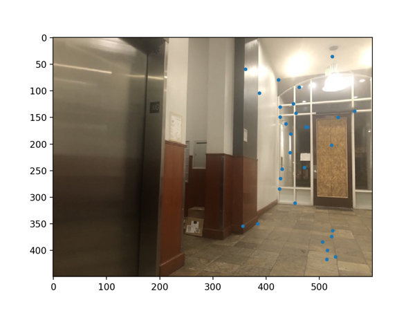
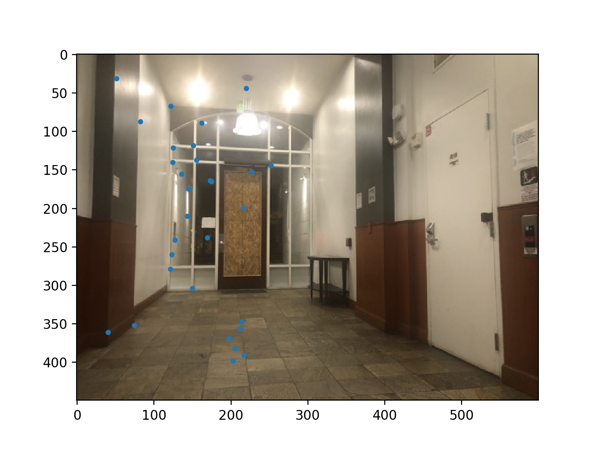
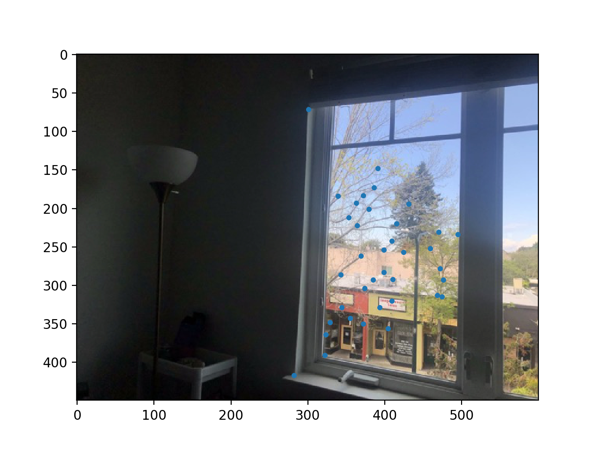
And here are the ones that I took for image mosaic.
Since I do not have a tripod, I used my arm as a tripod (I put my elbow
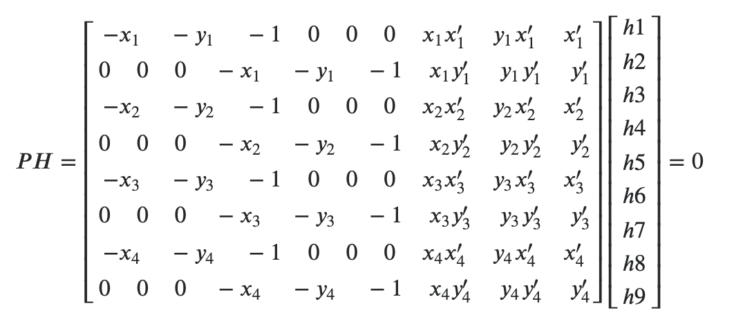
I used the following equation found online for reference. I got rid of the last column of P and h9, and defined the right hand side to be the negative of the last column of P. This is to avoid python giving back a matrix of all zeros. I created an over-determined system by defining 8 corresponding points, and used np.linalg.lstsq to compute the homography matrix.
For this part, I defined a python function to warp a given image according to a homography matrix. Since some pixel locations will map to negative coordinates, I expanded the canvas size to be 1.5 times as before on each side. And because the original warped image might be bigger than the original image, which can result in pixels with no values, I also downsampled the warped image every 2 pixels.

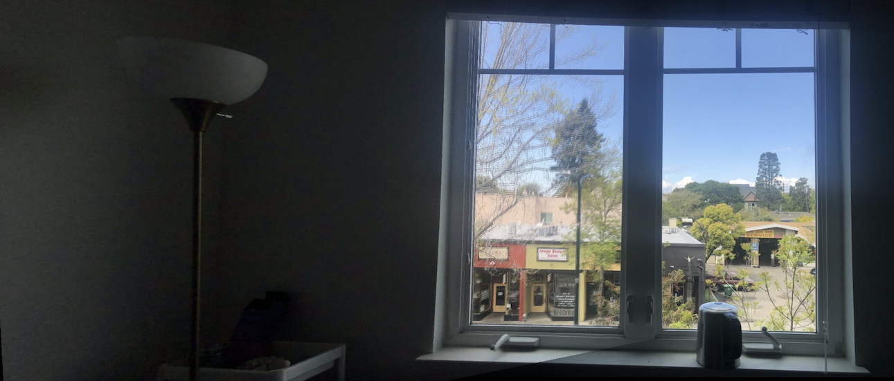
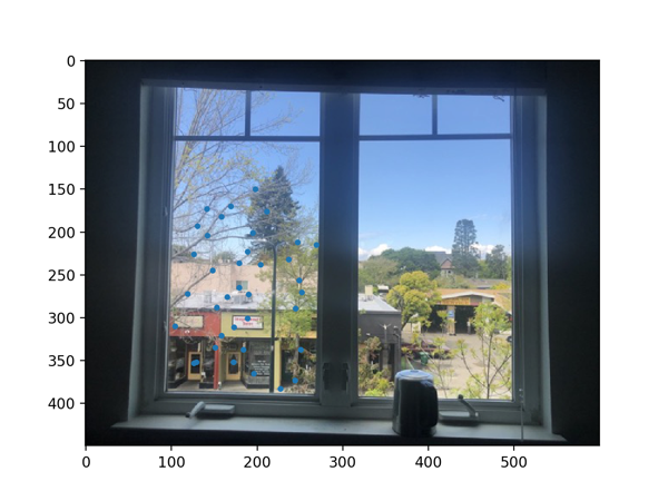
For the outdoor mosaic, I defined the points to be: white car wheels' centers, blue car wheels' centers, and the four corners of the shopping window. I warped both images. For the building mosaic, I defined the eight points to be the four corners of a wood panel and four corners of the door, and I warped the first image to the second. For the window mosaic, I defined the eight points be the corners of the window as well as those of the smaller rectangle on the window.
I identified the start and end x coordinates of the overlapping regions, and defined an alpha channel over that region to blend the two images. i.e. The alpha value decreases from 1 to 0 linearly in the overlapping region from left to right, and each column's pixels are defined by alpha * warped_im1 + (1 - alpha) * warped_im2.
However, we can see that the outdoor and the window mosaic gets a little blurry at the tree. I believe this is partially because my arm was not steady enough, and the window was a close object, and partially because Berkeley was windy and the branches shook as I was taking the picture
I learned from this assignment how cool homographies are, and how we can use an overdetermined system to reduce the risk of getting an error.
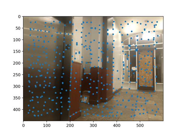
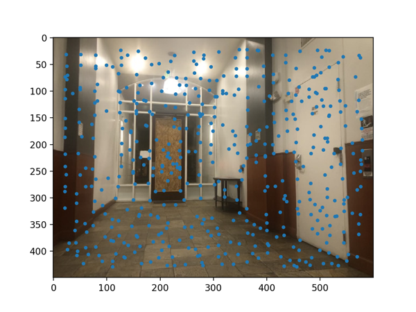
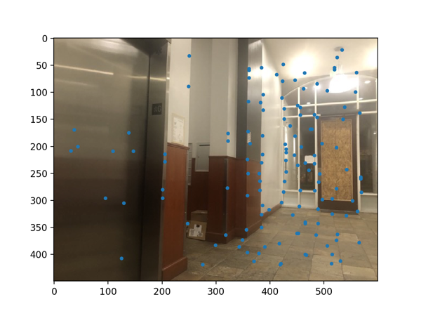
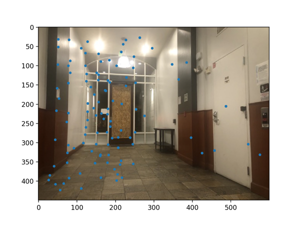
First, I detected corner features in the source images by using Harris Interest Point Detector (code from Professor Efros). Here are the results.
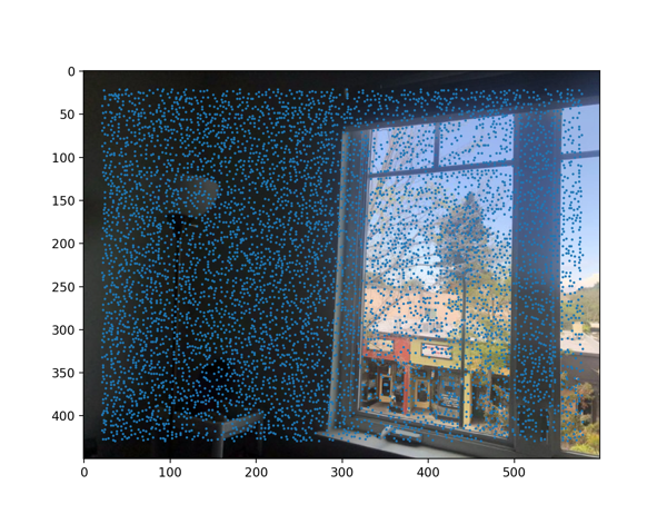
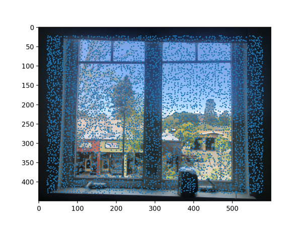
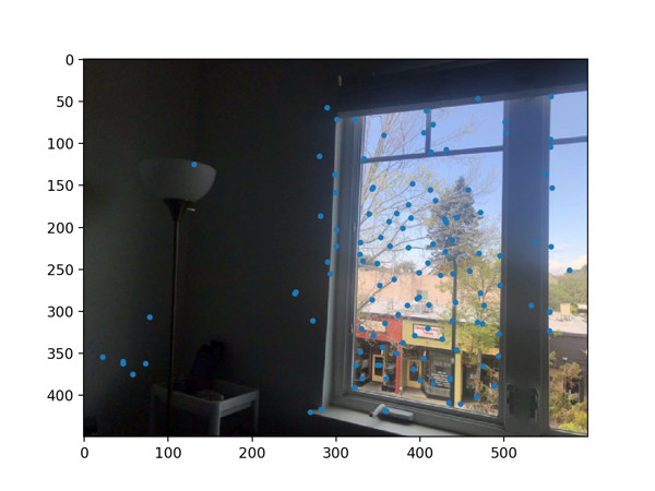
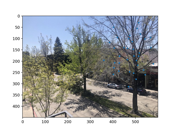
We then calculate the minimum suppression radius for every interest corner point and take the top 500 points with the maximum minimum suppression radius. Here are my results.


For this part, I extract a description of the local image at every point of interest after reducing the number of points of interest with Adaptive Non-Maximal Suppression. As specified in the spec, I did not worry about rotation-invariance, and instead just extracted 40x40 patches and downsampled them to 8x8. After that, I normalized the patch by subtracting the mean and dividing by the standard deviation.
To match feature descriptors, I created two matrices for the two images I'm trying to match. Each matrix is 500x64, with each row being a flattened feature descriptor. I used the dist2 function in harris.py to speed up the computation. The resulting matrix is 500 x 500, where the entry at the ith row and jth column is the difference between ith feature of the first image and the jth feature of the second image. For each feature in the first image, I find the errors of the best match and the second match and compute their ratio. If that value is below some threshold (which I chose to be 0.6), then I keep the best match as a pair of features. This is based on Lowe's approach.
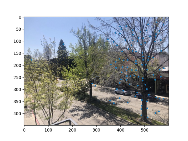
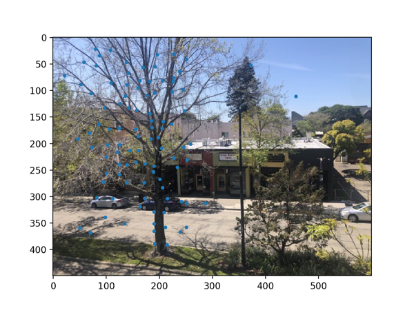

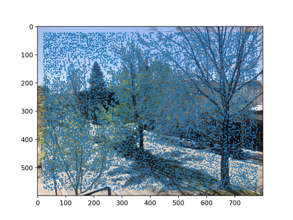
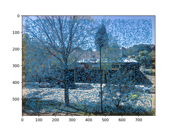
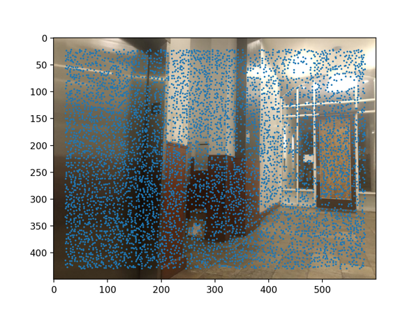
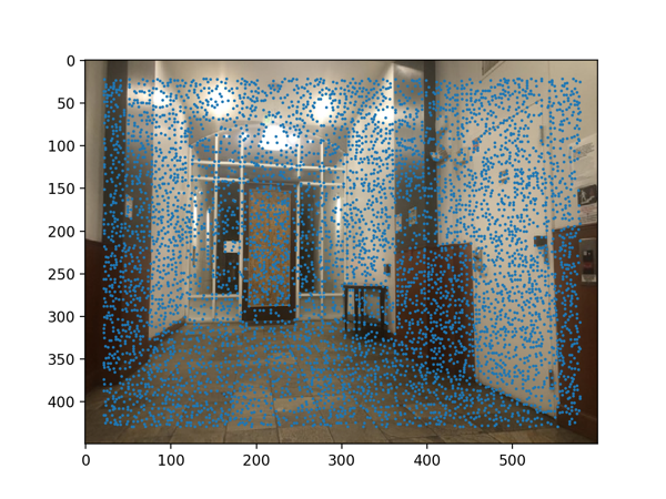
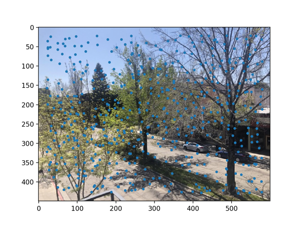
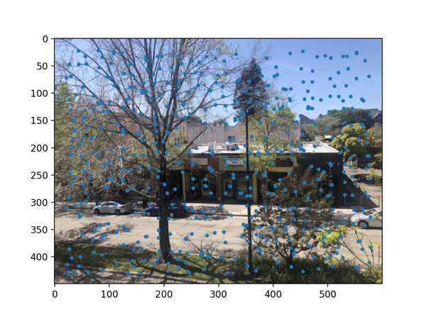
This step is to further eliminate outliers. For this part, I implemented RANSAC. For each iteration, I randomly sample 4 pairs of matching feature points and calculate an exact homography matrix. Then I take all the feature matching points of the first image and transform them with this matrix, and compare the transformed coordinates with the feature matching points of the second image. If the squared difference is less than 0.6, then we say this point is an inlier. We repeat this process 1000 times, and keep the largest set of inliers. Then we compute the final homography matrix based on this largest set. Here I plot the largest set of inliers.
Manual mosaics are on the left column while automatic ones are on the right. We can see that automatics ones do significantly better at aligning the trees. While the trees in the manual mosaics are blurry, they are not at all blurry in the autowarped version. This is because the automatic feature extraction tends to select feature points on the tree branches, thus making them align better.