|
|
|
|
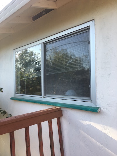
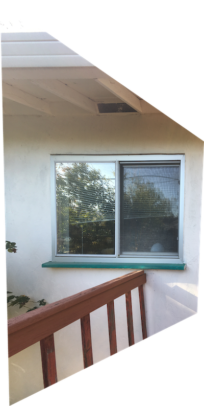
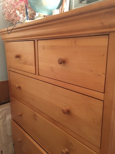
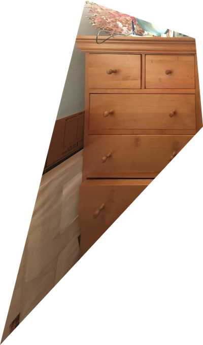
For this part of the project, we transformed images with a homographic transformation to rectify an image or combine images into a mosaic.
To recover the homographic transformation H, we use multiple correspondence points with the idea that Hv = u where v = [p1x, p1y, 1] and u = [w * p2x, w * p2y, w] and (p1x, p1y) corresponds to (p2x, p2y) of the desired end position. Some algebra tells us that if we write H into a flattened vector of [a b c d e f g h], p2x = (a * p1x + b * p1y + c - g * p2x * p1x - h * p2x * p1y) and p2y = (d * p1x + e * p1y + f - g * p2y * p1x - h * p2y * p1y). We can now write out a matrix vector equation and then use least squares to solve the problem given a set of correspondence points.
To warp an image, we must first construct a polygon of the warped final shape of the image, then use the inverse of H to get the matching coordinates for the unwarped image to the warped version. I also used a RectBivariateSpline to prevent jaggies or other undesirable aliasing effects.
|
|
|
|
|
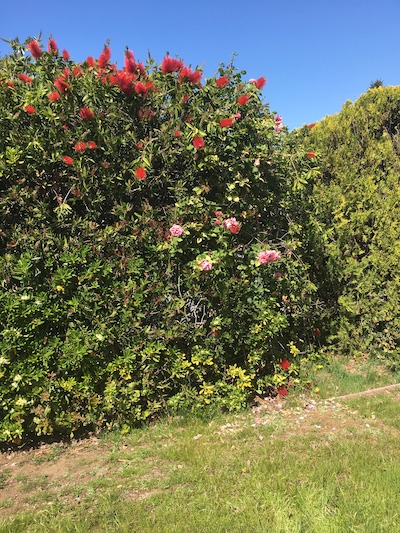
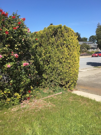
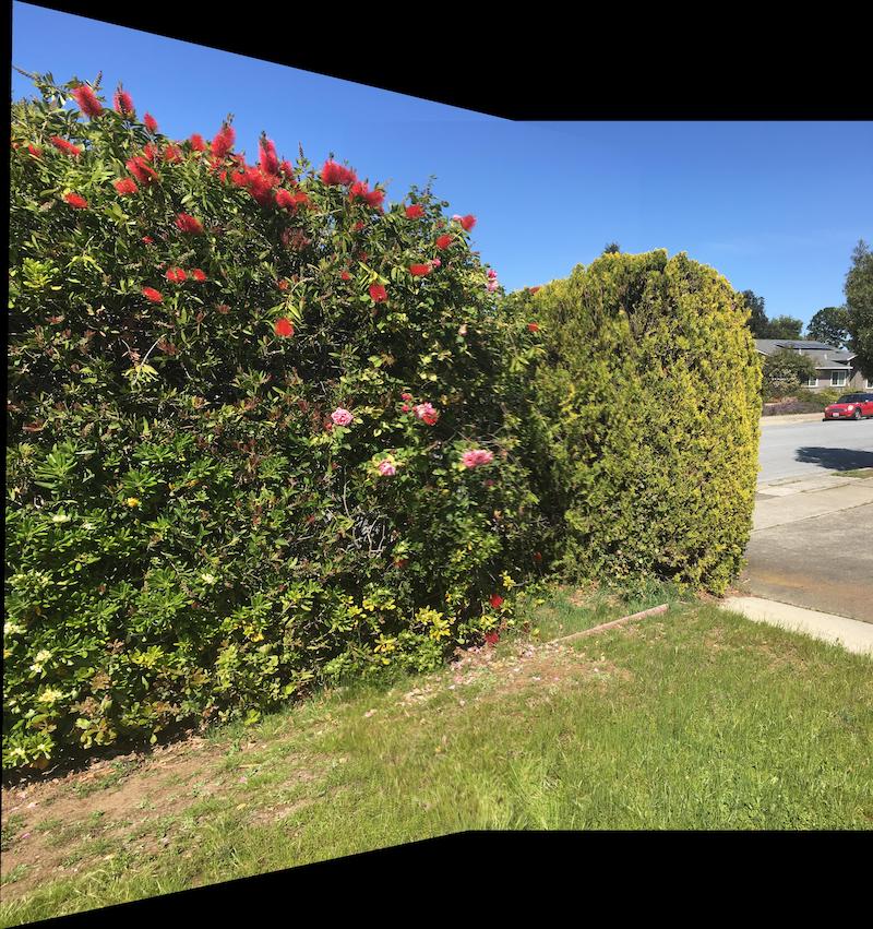
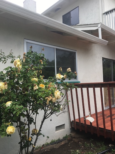
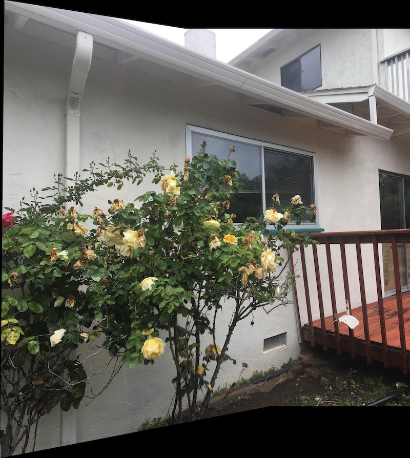
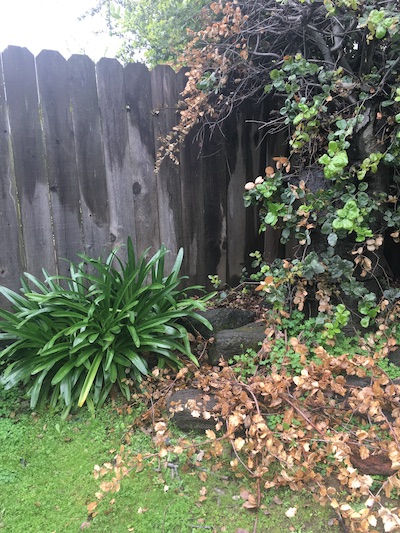
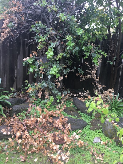
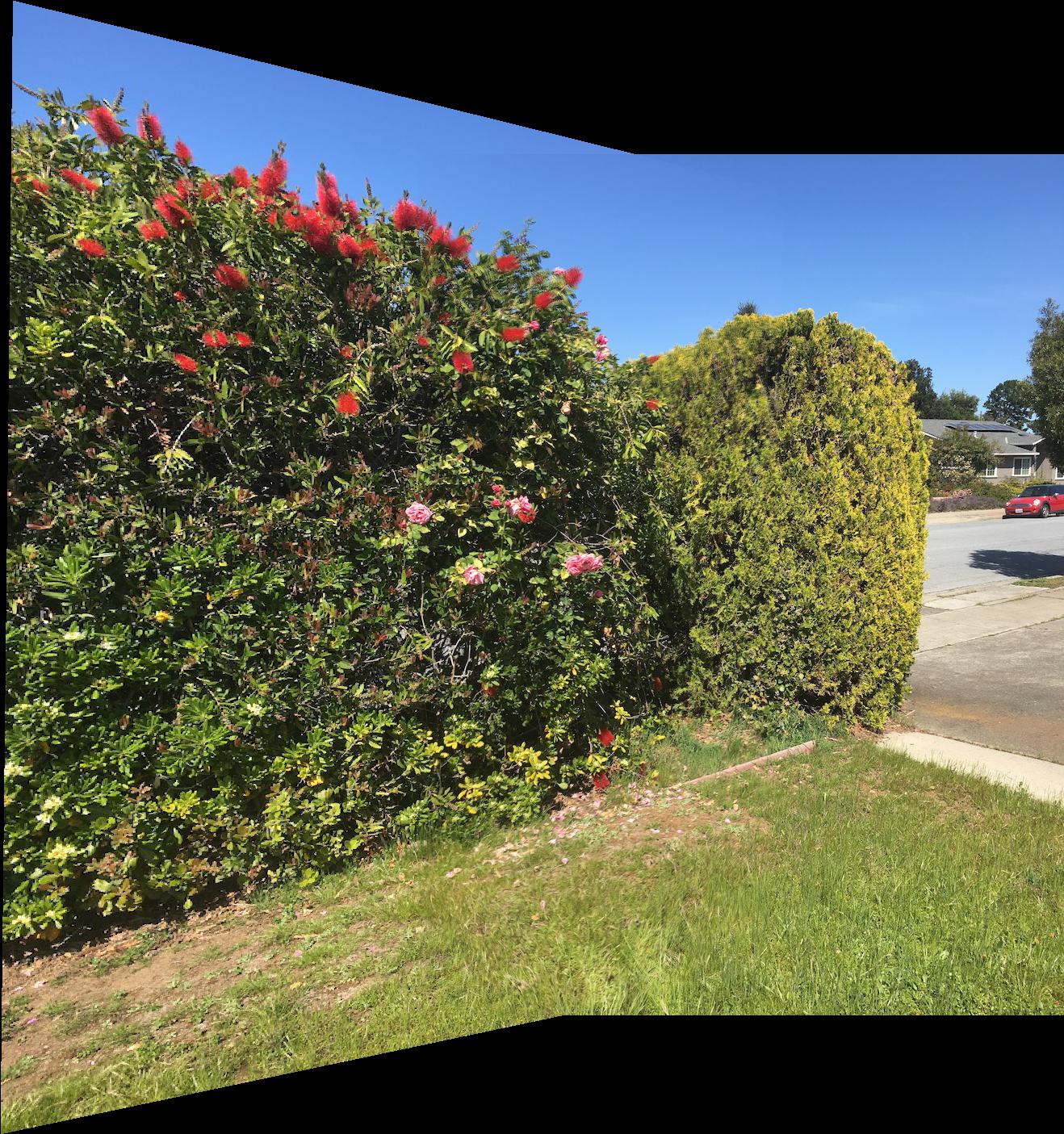
To merge images into a mosaic, I warped one image into the plane of the other image. As edges were extremely obvious when I just overwrote one image with another, I constructed an weighting layer for both images that would be 1 at the center of the image and fall off based on the distance of the position to the pixel. I then merged the images together using weighted averaging.
|
|
|
|
|
|
|
|
|
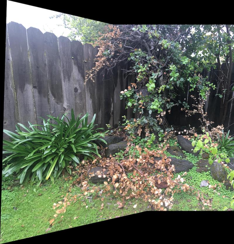
In this part of the project, I automatically matched, warped, and merged two images into a mosaic. The second two steps come directly from the first part. The first step, matching, involved four main steps: getting Harris points that are easily identifiable and spread across the entire picture, extracting feature descriptors, matching features based on the squared distances between the pixel values of the feature descriptor windows, and using RANSAC to compute the optimal homographic transformation.
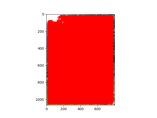
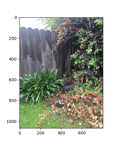
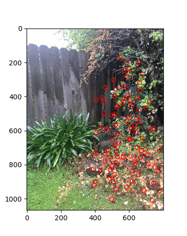
I used the starter code to find all possible Harris points or "corners", which means having the largest change in both the x and y direction. In accordance with the starter code, I excluded the Harris points along the edges:
|
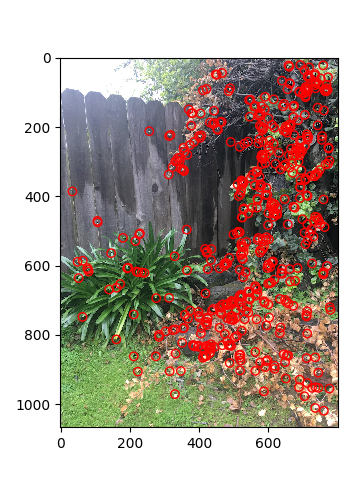
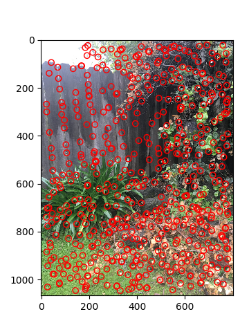
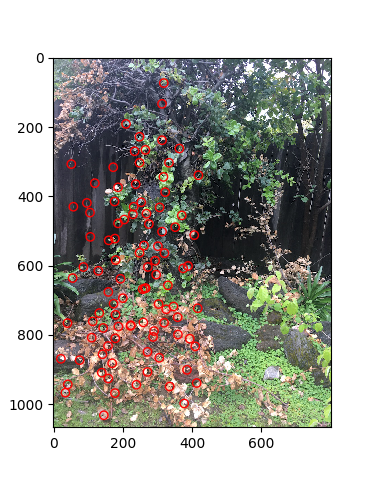
To select the most optimal Harris points, I wanted to include ones that are easily identifiable and also spread across the entire picture. To do this, I implemented Adaptive Non-Maximal Suppression as explained in the paper. I first found the distances between every Harris point. Then, for each Harris point, I found the minimum distance or "radius" by which it is the "largest" (or its Harris value is no less than some constant c times the Harris value for all points in that circle). We select the Harris points with the biggest circles in which it is comparatively large. Below is a comparison between just selecting the 500 points with the largest Harris values and using adaptive non-maximal suppression to select 500 points:
|
|
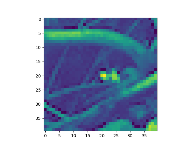
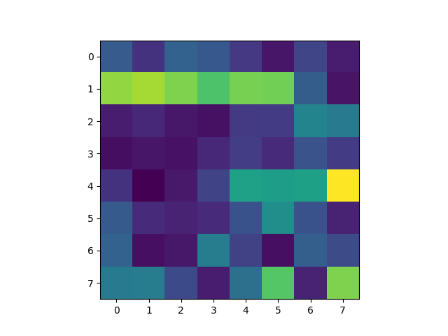
I selected 40 pixels around each Harris point and convolved each window with a Gaussian blur of size 5x5 pixels. After bias/gain-normalizing by subtracting the mean value and dividing by the standard deviation, I selected every fifth pixel to end up with a 8x8 window for each original 40x40 window.
|
  |
To match features together given the feature descriptor windows from the previous step, I flattened each window to get a vector of dimension 64. I then got the squared distances between each vector of the first image compared to each vector of the second image, which is equivalent to getting the squared difference between the pixel values for each possible pair of feature descriptors. Then, for each feature, I got the corresponding feature with the smallest squared difference in the other image. Of course, we may have cases where the feature descriptor has no corresponding descriptor in the other image or we are not certain the pair is good. To get around this, I used the idea that either the first one is way better than the second option or else it is no good at all by comparing the minimum squared difference against the second minimum squared difference and seeing if the min is much smaller. Only then would I keep the pair.

|
|
I implemented the RANSAC loop as described in lecture. In each loop, I selected four random points (the minimum number of points required to compute a homographic transformation matrix), computed the matrix, and then found all the inliers (aka feature coordinates which when transformed are close to the corresponding coordinates in the other image). I repeat this, keeping the largest set of inliers at each loop, for a large number of times (2000 times, though 1000 was pretty good already). Finally, I computed a least squared approximation of the H matrix using the largest set of inliers.
|

|
|
|
|
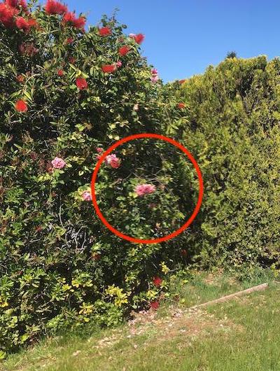
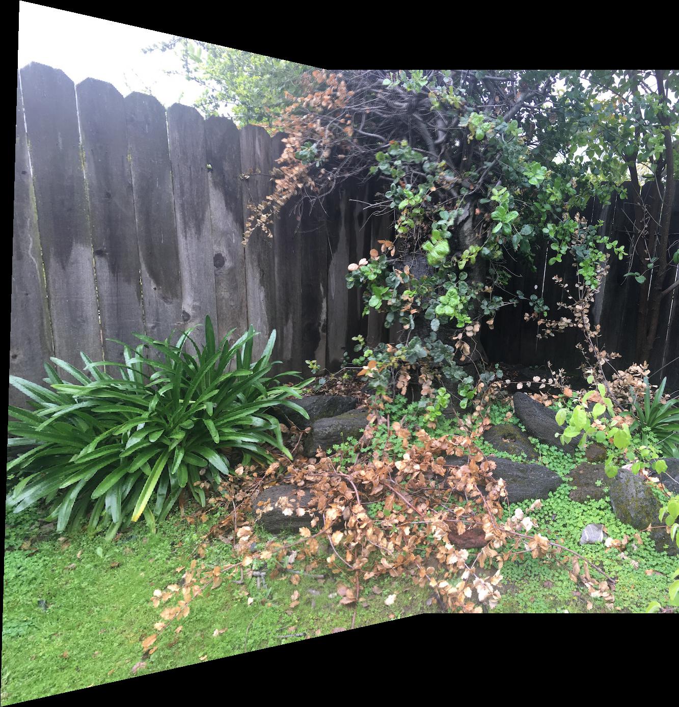
Comparison
|
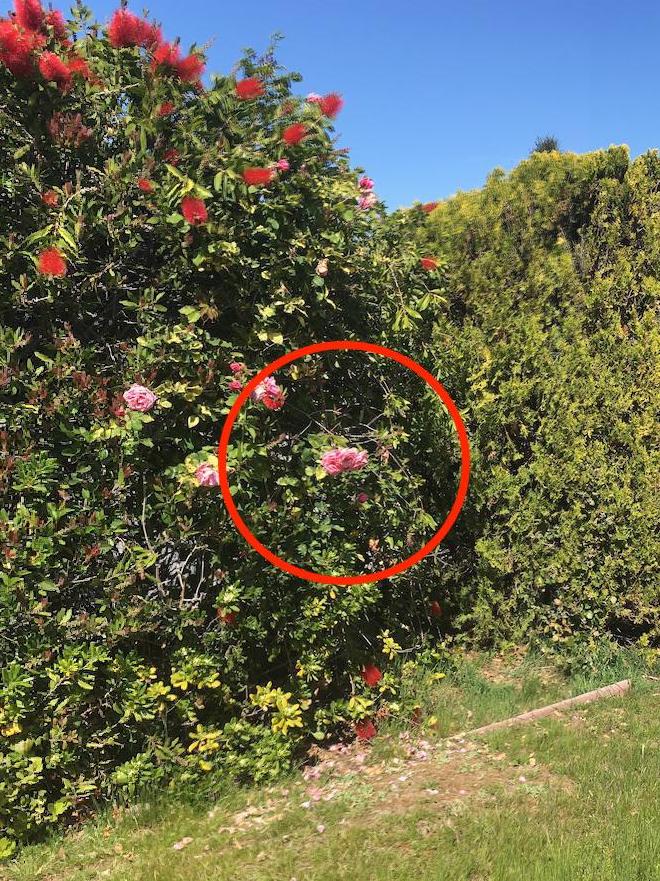
|
Notice how the flower in the center of the circle for the hand selected version is slightly blurry. It is clearer in the automatic version
|
|
|
|
|
|
There was a very slight improvement in quality of matching from using automatic instead of hand matching, except for the bushes, which was a little more apparent. The reason for this is most likely from how I gave up on using ginput and instead used my art tool (Medibang Paint Tool) to zoom in on pixels and nearly perfectly get the exact corresponding coordinates. I got 16 points for each image, which is pretty stable. As a result, my hand matched ones were already pretty well done, so I am quite satisfied with how the automatic version performed even slightly better than what I did, and much quicker (from nearly half an hour per pair of pictures via hand matching to less than a minute per pair via automatic matching).
The coolest thing I learned was the fact that rotations do not bring in any new information and hence can be computed via homographies. I found it extremely cool when I rectified the image and it almost appeared as though I just took another picture just at a different angle. I also found the adaptive point selection to be quite interesting and elegant once I understood what the paper was trying to say.