Image Warping and Mosaicing

Introduction

In this project we explore how to create panorama images! Specifically, we will take photos with the same point of view but with rotated viewing directions and with overlapping fields of view. Using point correspondences to recover homographies from the one image to the other, we can then perform a projective warp and blend the results together to create a panorama.

Pictures!

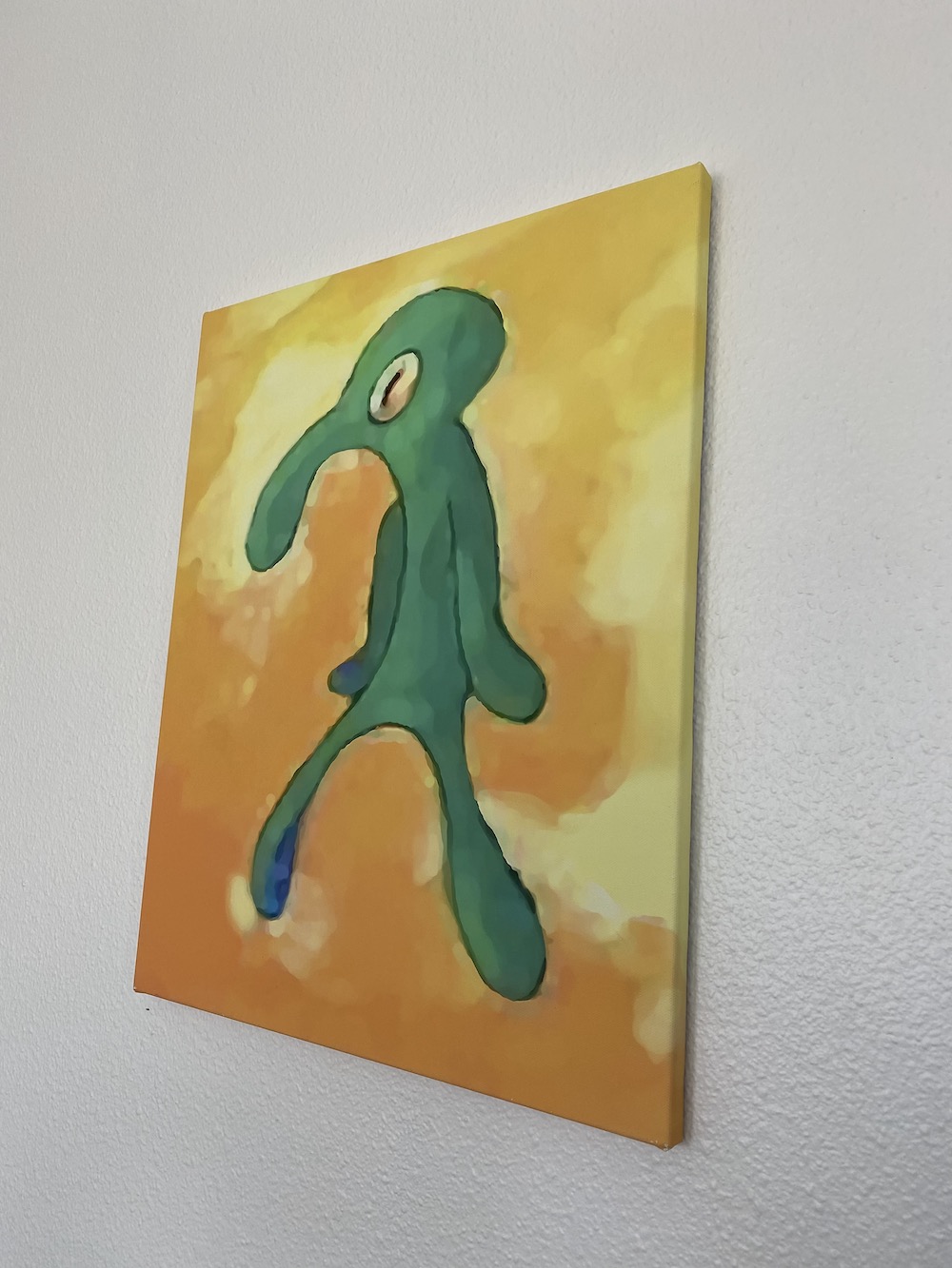
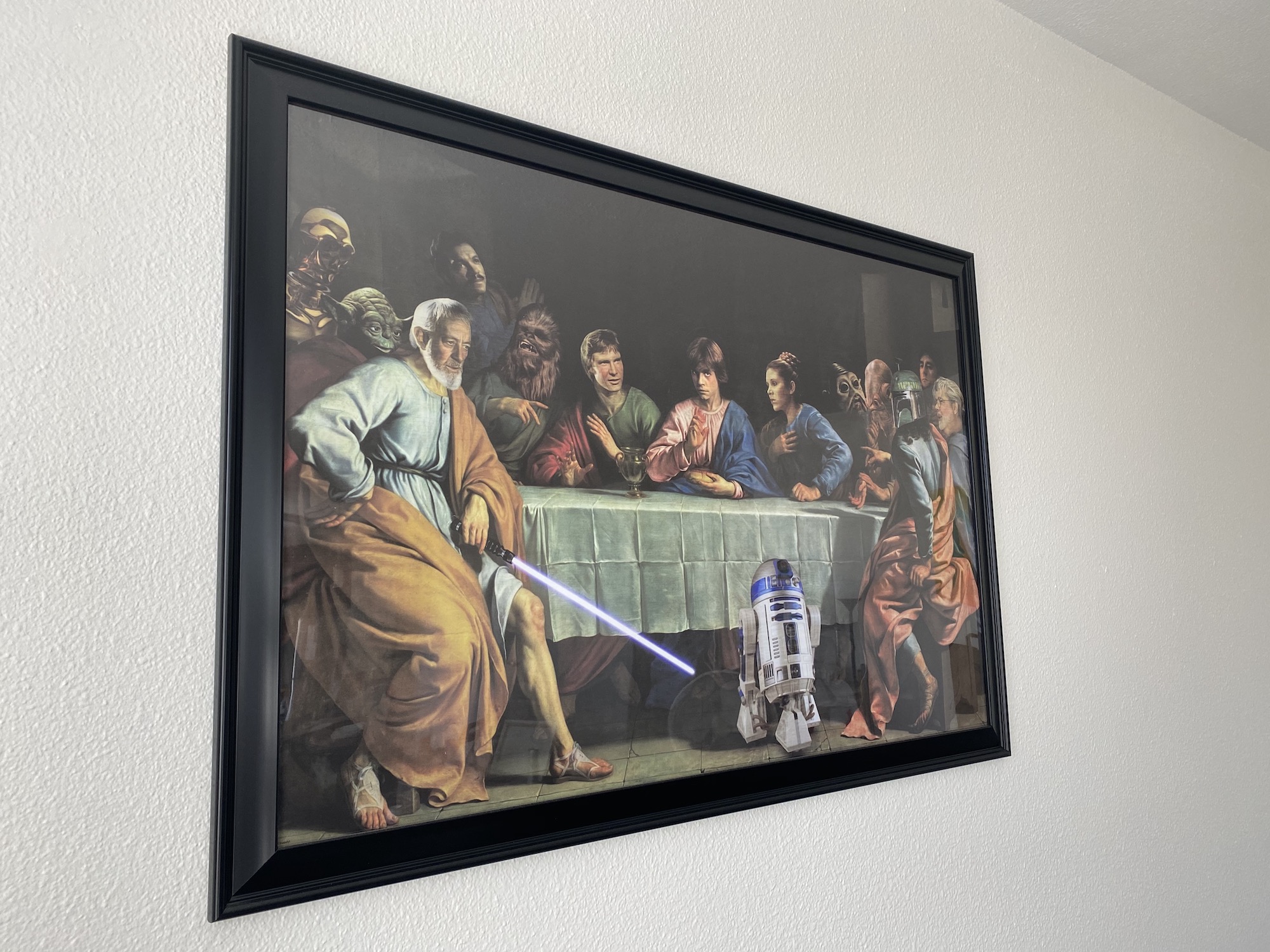
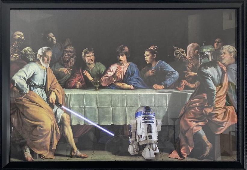
In order for this to work, we need some well taken pictures. Unfortunately, I don't happen to have a tripod at my disposal and we're under quarantine. That being said, I did my best to take some pictures using my smartphone.

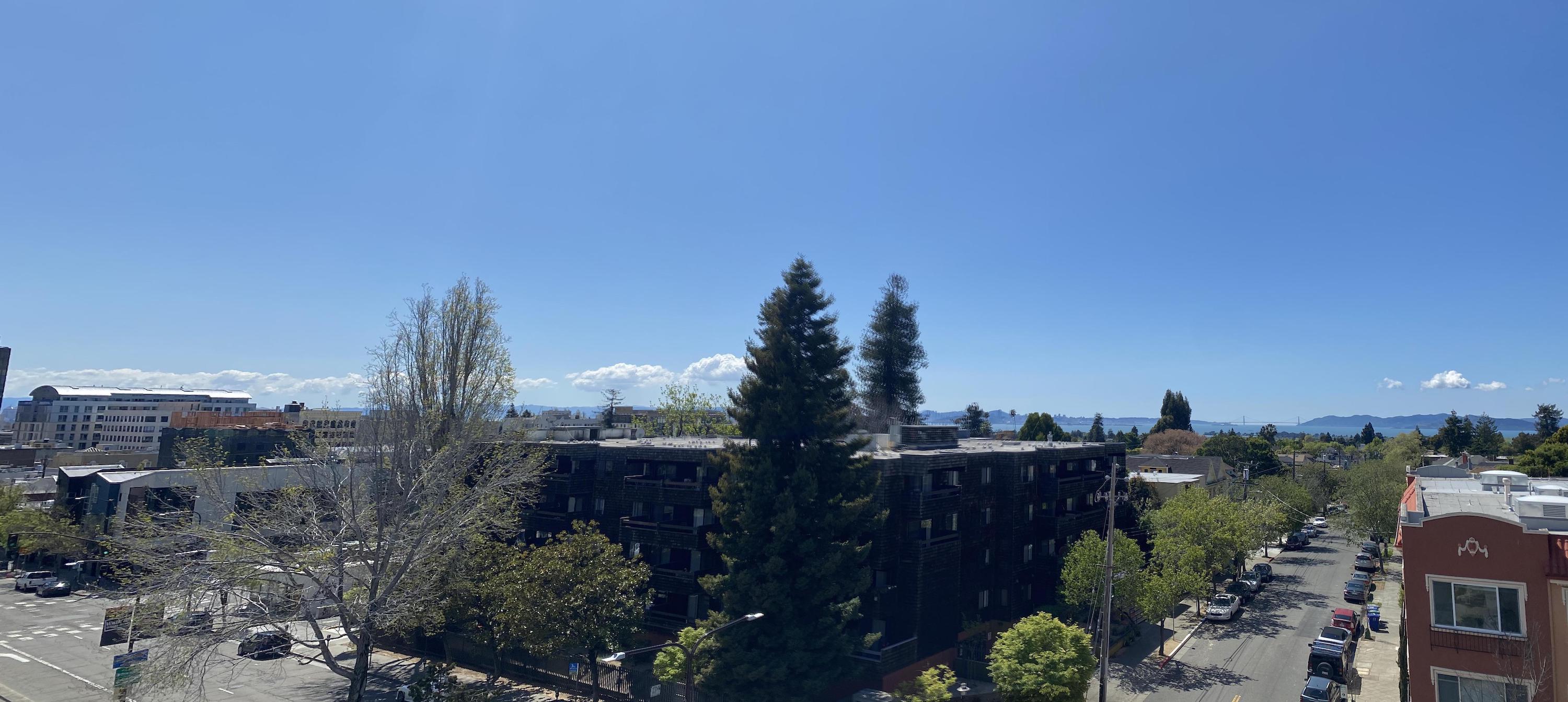
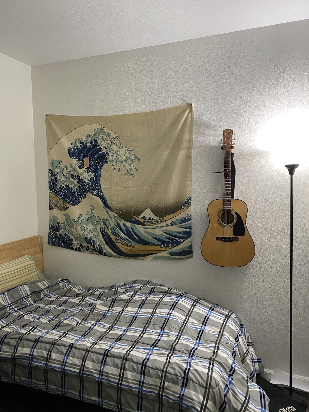
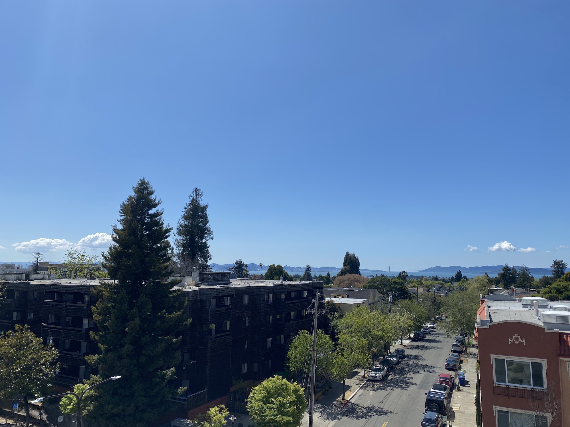
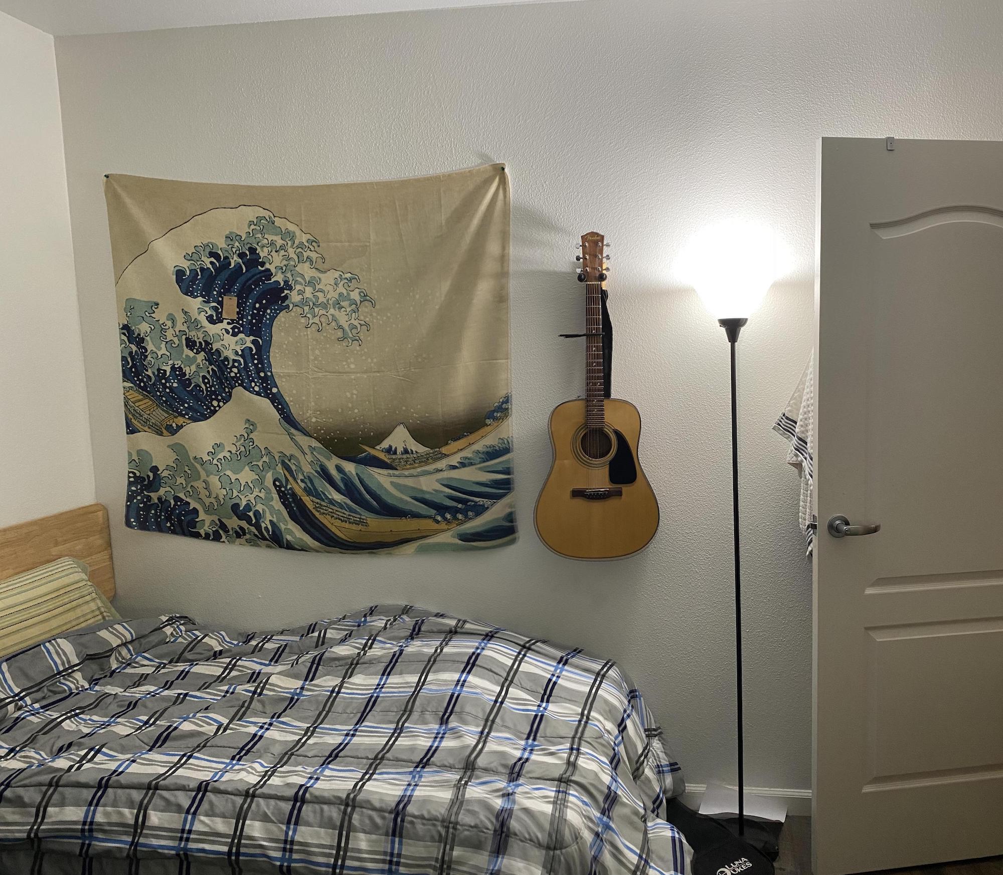
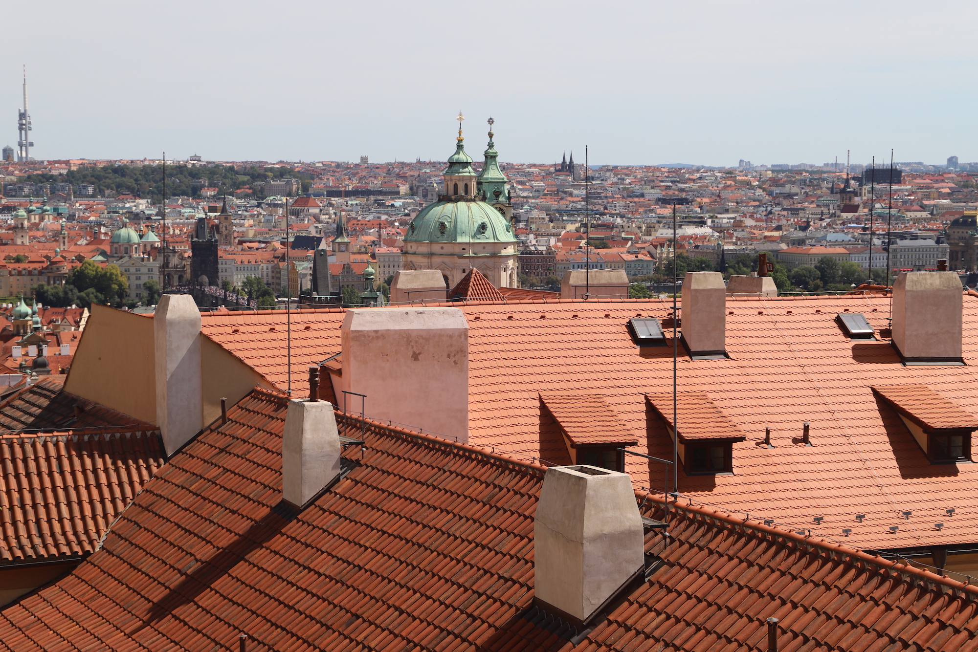
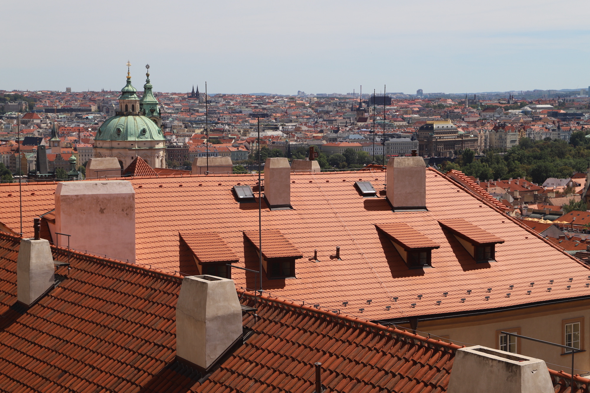
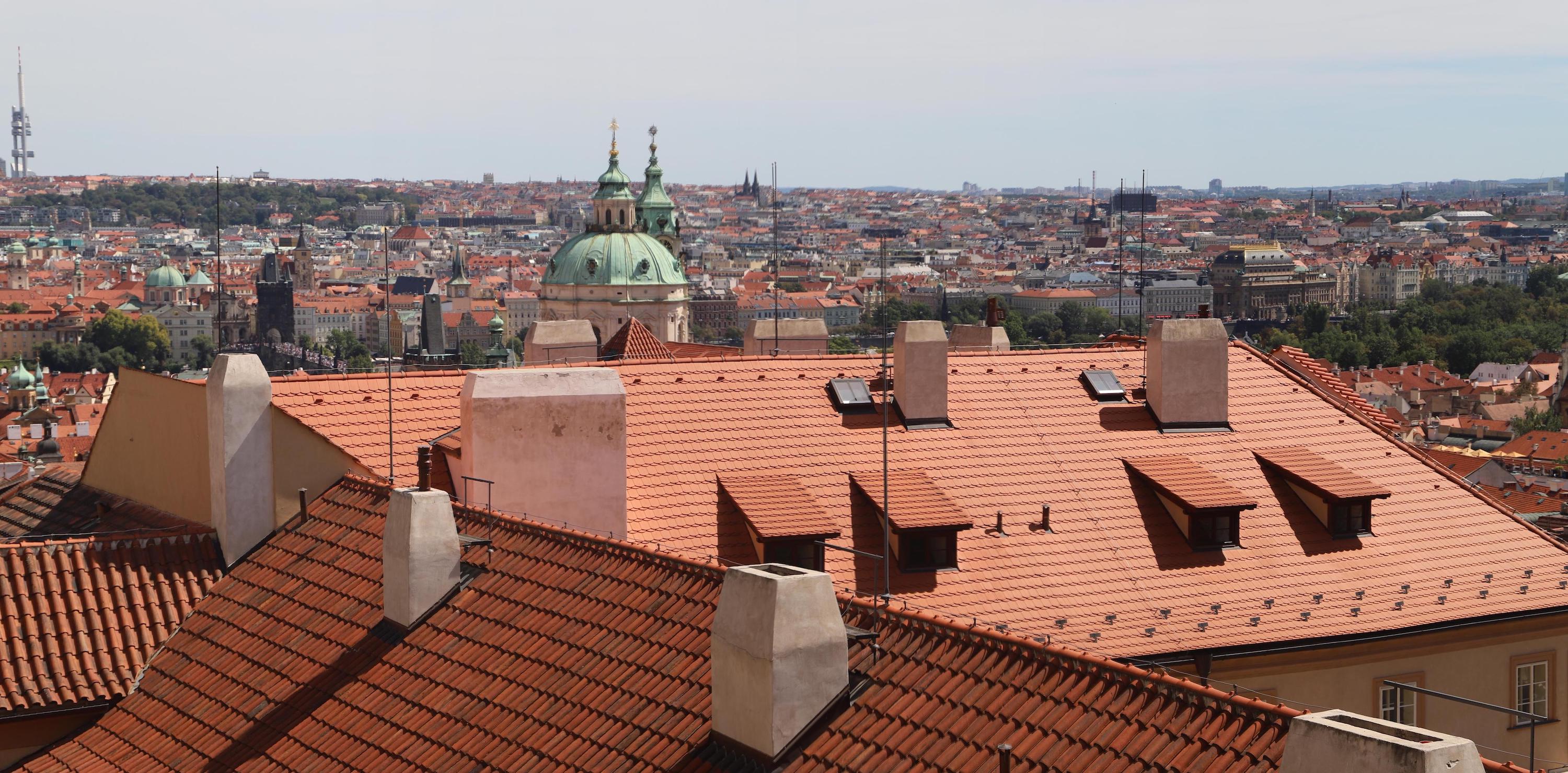
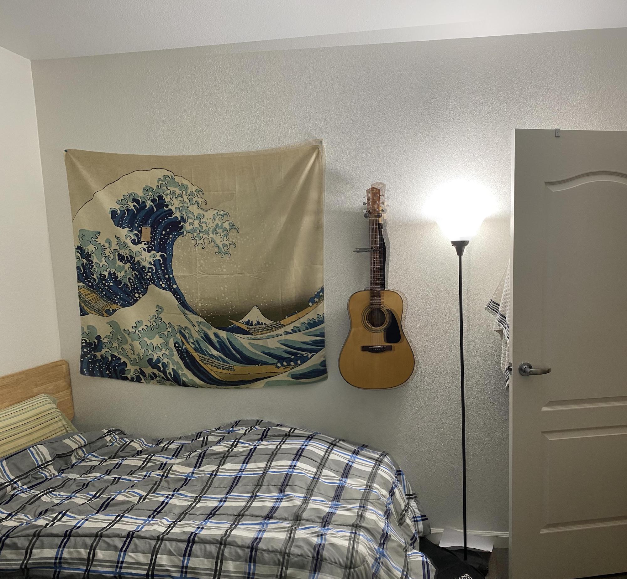
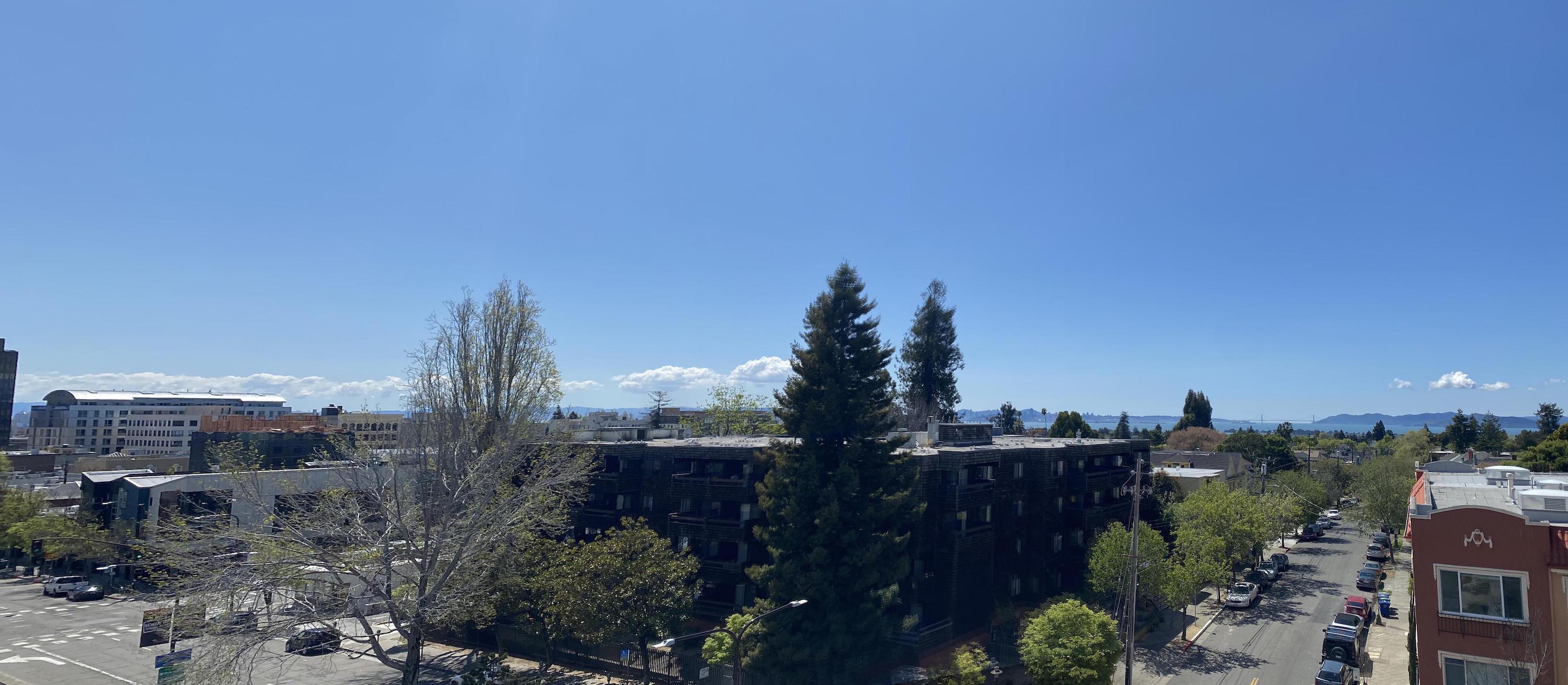
I took some pictures of my room in my apartment and the view from out on my balcony from the same point of view but with different viewing directions, making sure that each pair of pictures had a substantial amount of overlap.

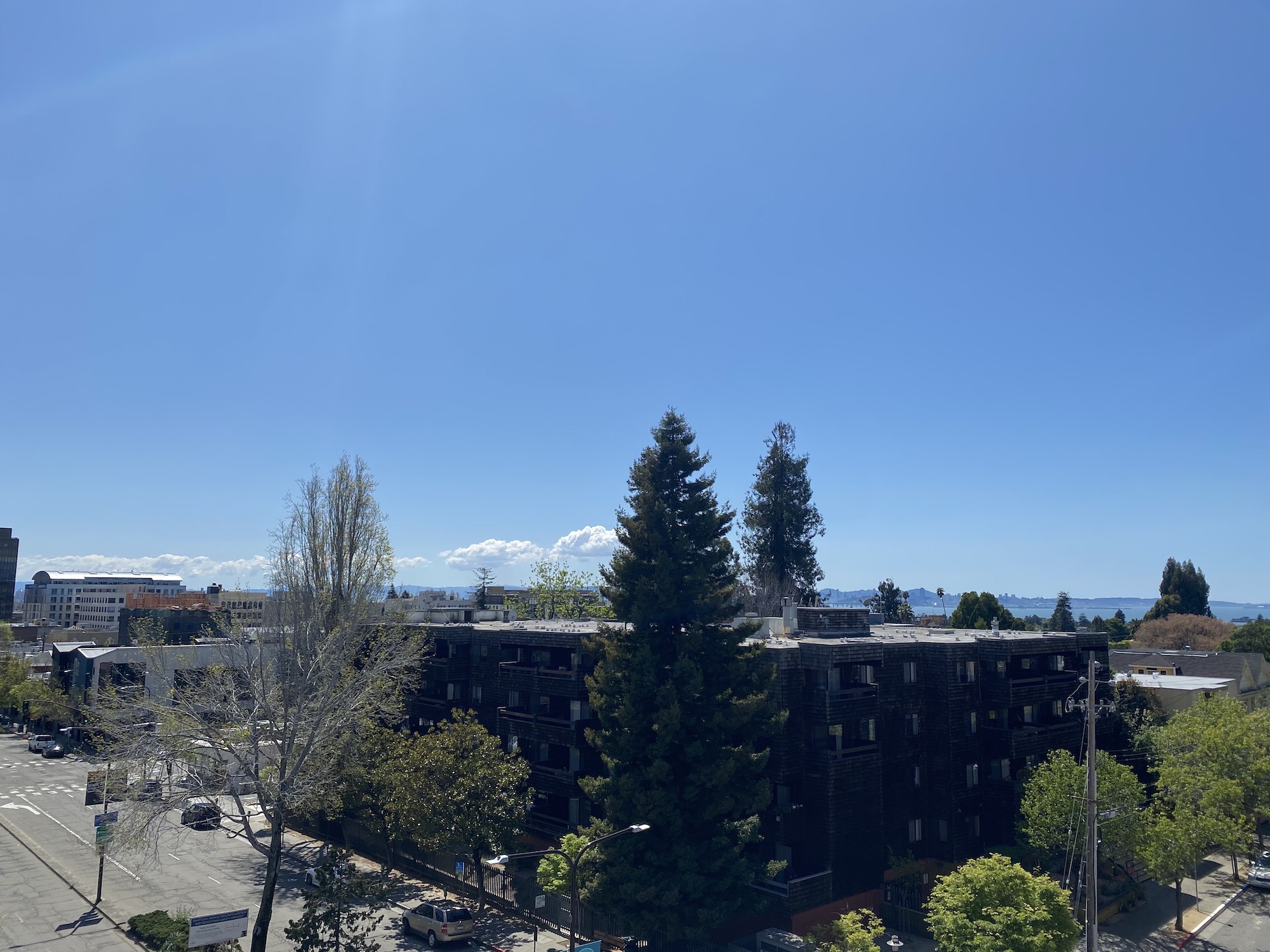
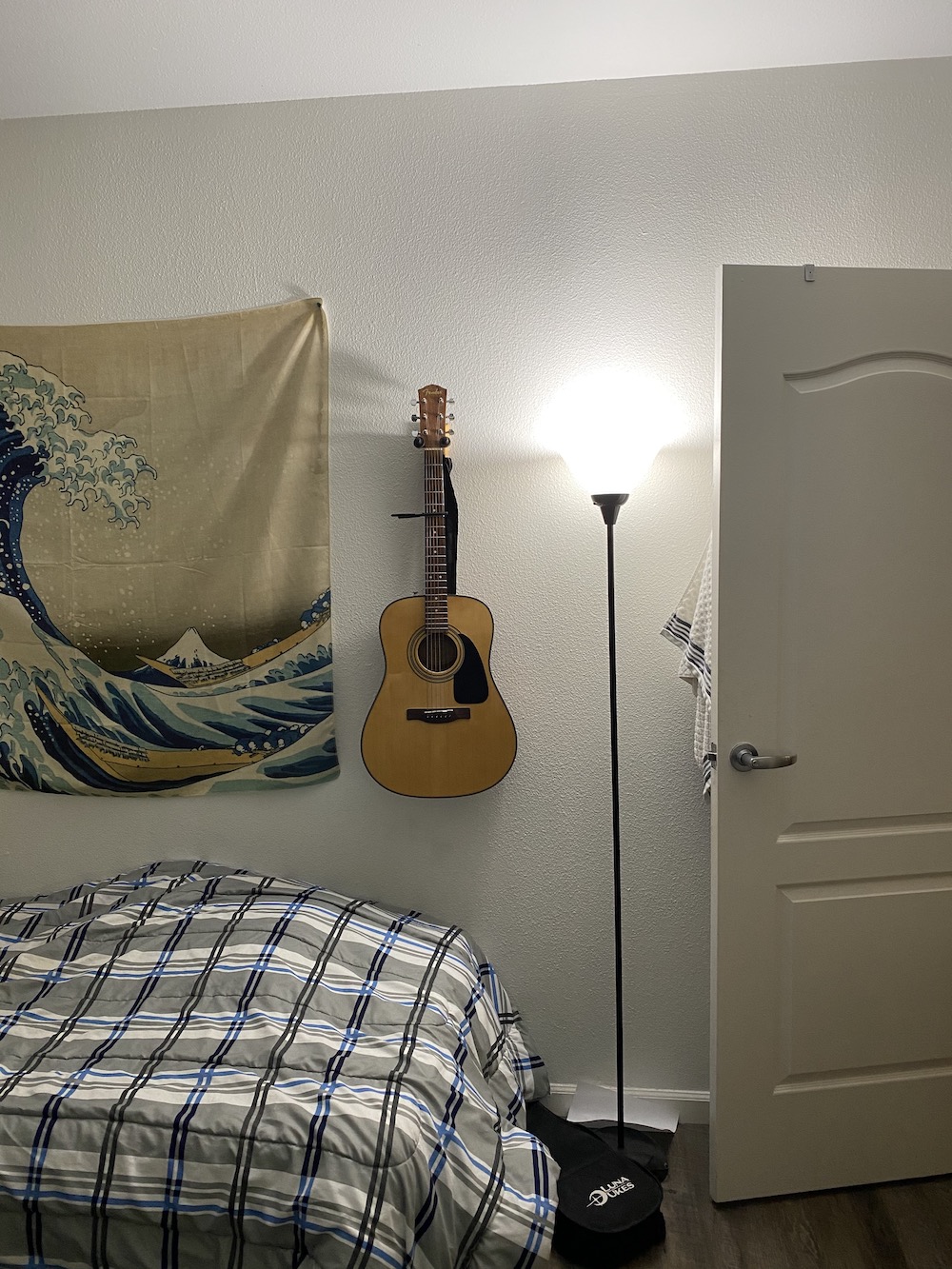
Before beginning to think of how to combine the two images into a panorama, we must define pairs of corresponding points on the two images by hand (yes, this can unfortunately get quite tedious). After defining pairs of corresponding points between the two images, we move on to the next part...

Recovering Homographies

Given the set of corresponding points between two images, we can relate the two according to the transformation $Hp = p'$ where $$H = \begin{bmatrix} a & b & c\\ d & e & f\\ g & h & 1 \end{bmatrix},$$ $$p = \begin{bmatrix} x_1 & & x_{n}\\ y_1 & \cdots & y_{n}\\ 1 & & 1 \end{bmatrix},\ \ p' = \begin{bmatrix} wx'_1 & & wx'_{n}\\ wy'_1 & \cdots & wy'_{n}\\ w & & w \end{bmatrix} $$ Thus, we have $8$, unknowns which we are trying to solve for with $n > 8$ equations. Since we have an overdetermined system, we will need to use a leas squares approximation to solve for the values of $H$. With some algebra, it can be shown this is equivalent to solving $Ax = b$ which can be written as the following: $$ \begin{bmatrix} x_1 & y_1 & 1 & 0 & 0 & 0 & -x_1 x'_1 & -y_1 x'_1 \\ 0 & 0 & 0 & x_1 & y_1 & 1 & -x_1 y'_1 & -y_1 y'_1 \\ & & & & \vdots & & & \\ x_n & y_n & 1 & 0 & 0 & 0 & -x_n x'_n & -y_n x'_n \\ 0 & 0 & 0 & x_n & y_n & 1 & -x_n y'_n & -y_n y'_n \\ \end{bmatrix} \begin{bmatrix} a \\ b \\ c \\ d \\ e \\ f \\ g \\ h \end{bmatrix} = \begin{bmatrix} x'_1 \\ y'_1 \\ \vdots \\ x'_n \\ y'_n \end{bmatrix} $$ For the purposes of this project, I ended up using correspondences anywhere between $n\in[20,30]$.

Image Rectification

Now that we have solved for the homographies, we should be able to perform an inverse warp to fill in every pixel value in the desired output image based on the corresponding coordinates in the input as defined by the homography transformation.

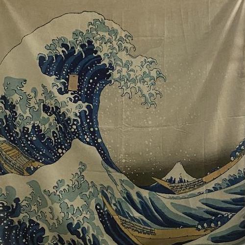
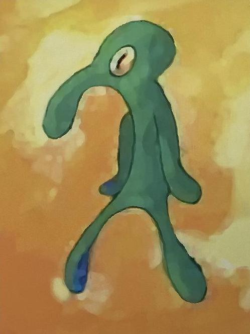
A cool application of this is image rectification! Here we take a few sample images with some planar surfaces, and warp them so that the plane is frontal-parallel. This is acheived by selecting 4 points representing the corners of the plane in the original image, and choose the correponding points in the output to be the corners of a rectangle. Here are some examples:

Mosaics

Now comes the challenge of building a mosaic (panorama) image! All we do is use the recovered homography between the two images and then warp one onto the image plane of the other. Then all that is left is to just blend the results together.

We just use a simple alpha blending on the resulting warps on the overlapping sections of the images. The results are shown below.

Automatic Stitching

Now comes the challenge of automatically building a mosaic (panorama) image without manually choosing correspondence points! In order to accomplish this task, we use a simplified version of the algoritm presented in the paper Multi-Image Matching using Multi-Scale Oriented Patches by Brown et al. to find the point correspondences. Once this has been completed, we proceed to blend the images together per the aforementioned methods.

Harris Corners

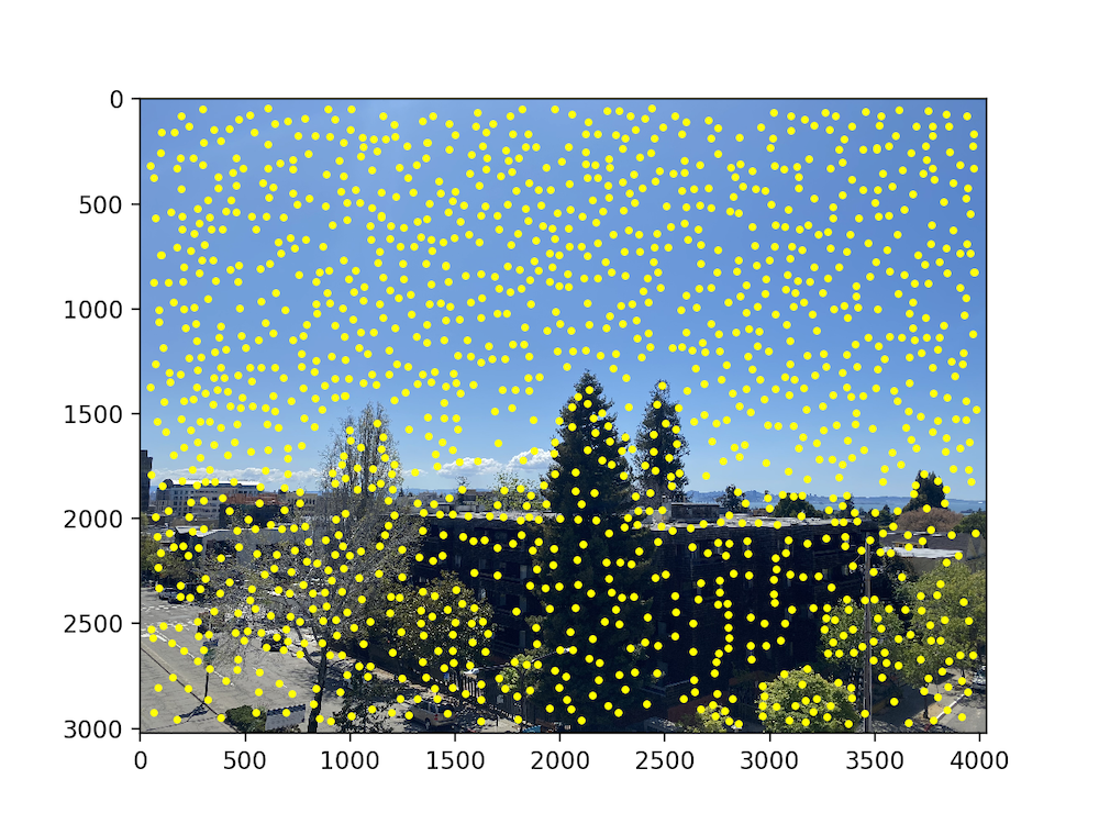
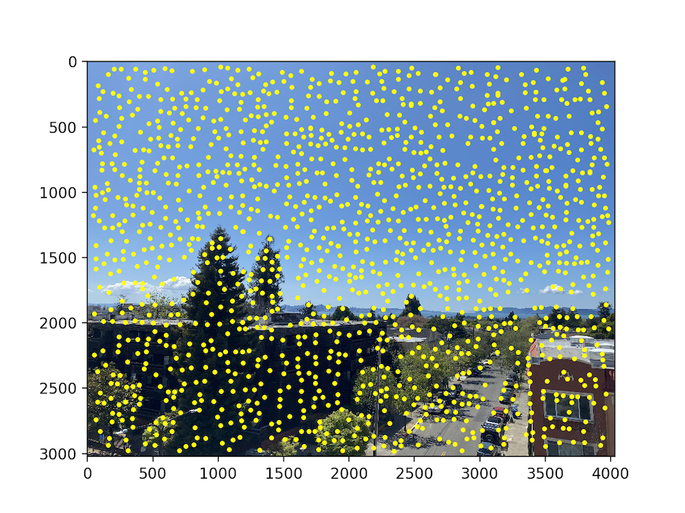
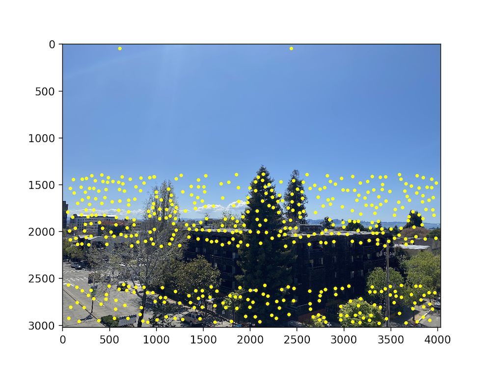
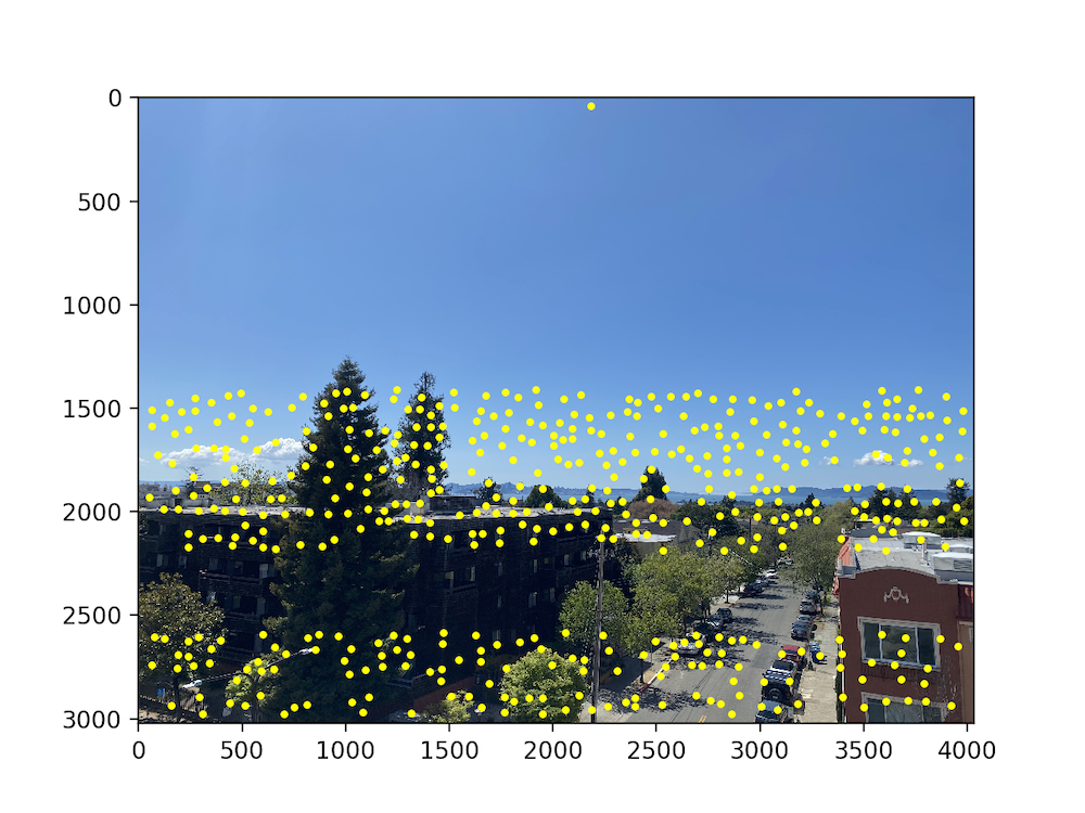
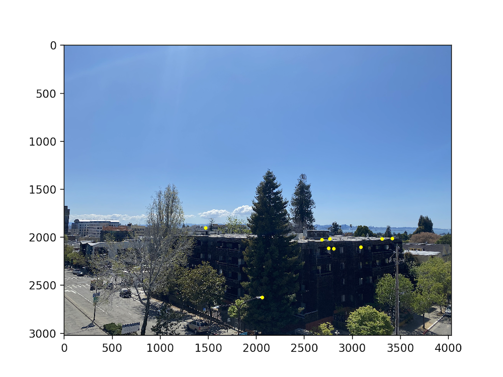
The first step in finding matches between images is to generate potential points of interest in the images. We use the provided Harris Corner Detector algorithm to do so. This returns a response matrix representing the corner strength at every pixel coordinate in the image (to be utilized in the later parts), and specific points of interest as seen below.

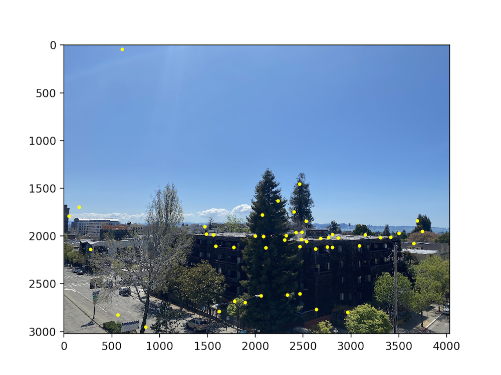
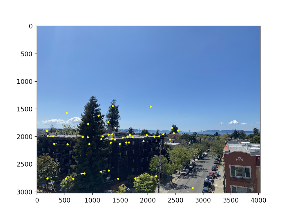
Adaptive Non-Maximal Suppression

As you can see above, there are still an incredible amount of points in the image. We want to limit the maximum number of points we want to choose, but we can't just randomly pick points to filter out. Instead we use an algorithm presented in the aforementioned paper called Adaptive Non-Maximal Suppression. The algorithm chooses the points with the top-$k$ values of $r_i$, the minimum suppression radius of point $x_i$: $$r_i = \min_{j} | x_i - x_j |, \text{s.t. }f(x_i) < c_{\text{robust}} f(x_j),\ \ x_j \in \mathcal{I}$$ where $\mathcal{I}$ is the set of all interest points retrieved from the Harris Corner Detector, and $f(x_i)$ is the response value of $x_i$. The results, with hyperparameters $c_{\text{robust}}=0.9$ and $k=500$ are seen below.

Feature Descriptor Extraction

Once we have determined where to place our interest points, we need to extract features for each point. These will then be used to determine a one-to-one point correspondence. As specified by the paper, we sample an 8 x 8 patch of pixels around the location of a given interest point, using a spacing of s = 5 pixels between samples. We then normalize and flatten this into a column vector to be used in the feature matching.

Feature Matching

Now that we have extracted the features for each point, we can begin to define one-to-one correspondences. For each point's feature vector in one image, we find the two nearest neighbors (i.e. two feature vectors of the other image closest in euclidean distance). We then decide whether or not to define a point correspondence between the given point and its nearest neighbor based on the the Lowe Ratio Test, that is we define the correspondence if nn1 / nn2 < thresh where thresh = 0.6 (as per my own experimentation). The point correspondences after feature matching are seen below.

RANSAC

After having found the point correspondences through feature matching, we notice that we still have some outliers. In order to reject such outliers, we use the RANSAC algorithm. I won't go through the details too much here, but I found that using 1000 iterations and a threshold of 0.5 worked relatively well. The final point correspondences are seen below.

Results!

Now we can finally blend the images together as we did before! Here are the auto-stitched results on the previously seen images.

Key Takeaways

Throughout the course of this project, we've touched upon all the difference mechanisms that go into stitching together images to form a panorama. I think it's really cool to see all the mathematics that goes into something we've all been doing with our phones and cameras since we were kids, and I hope you feel the same!