Introduction
In this project we will be taking a look at creating image mosaics from multiple overlapping images. In order to do this we will first have to collect images which we can go about converting into panoramas. We will then proceed first by computing correspondences between images manually. For this the corresponding features that exist in two images can be manually selected by hand. We will later create code which will instead automatically select these correspondence points for increased ease of use and accuracy of panoramas created. With this information we can then proceed to compute a homography between the images and then stitch the images together.
Image Warping and Mosaicing
Images
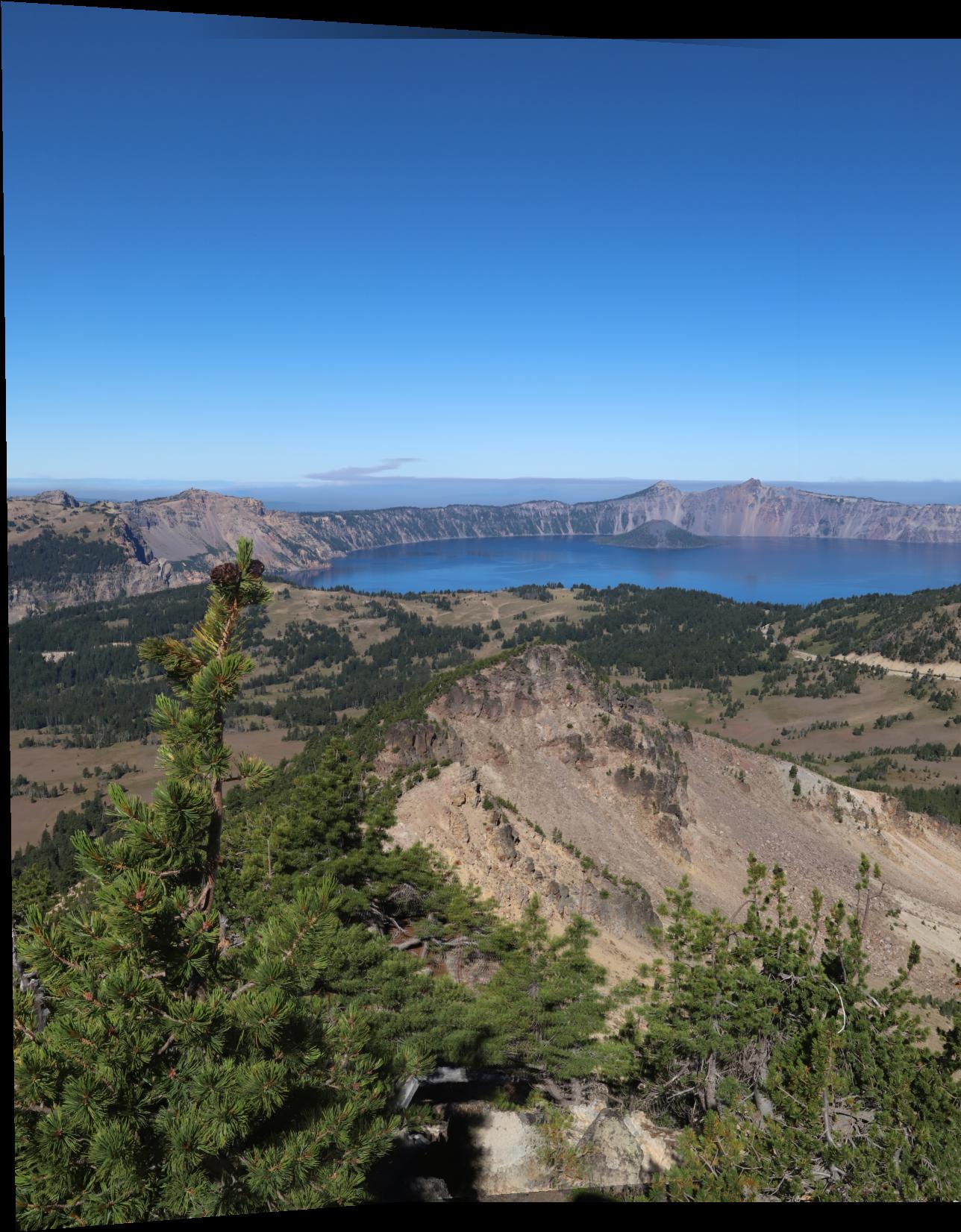
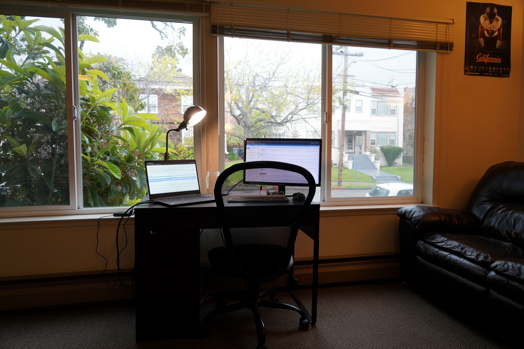
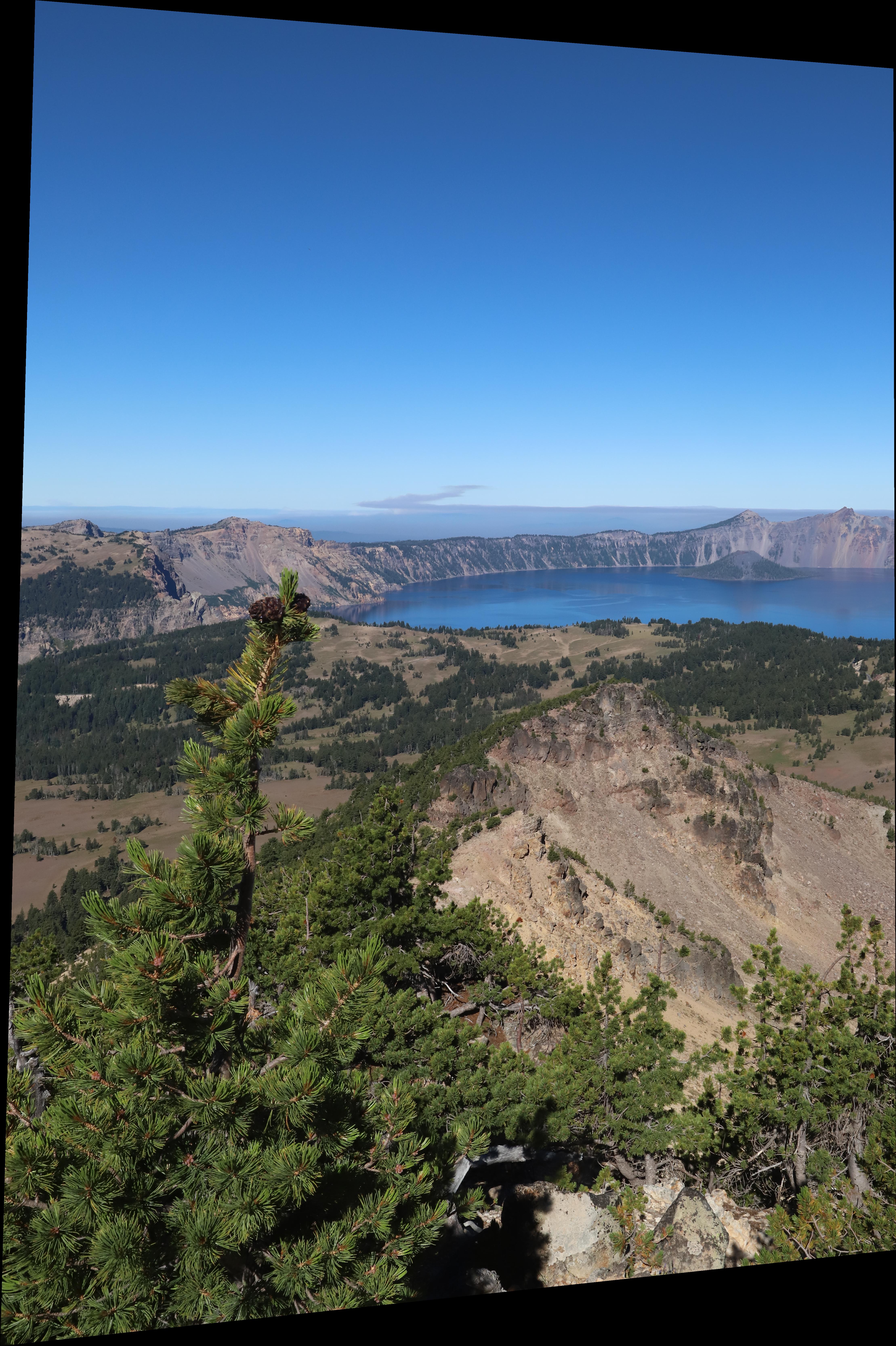
I will be using the following sets of three images for creating panoramas. Credits to the wonderful Shivam Parikh for the city and crater lake photos.


Recovering Homographies
We will be modeling the transformation from one image to another using a homography transformation \(H\) which will have the following form. $$H = \begin{bmatrix} a & b & c \\ d & e & f \\ g & h & 1 \end{bmatrix}$$
As we have 8 entries in this matrix, we have 8 degrees of freedom and we will need 4 points in order to determine this matrix. If we use only 4 points, slight variations and / or noise can lead to poor results. A better approach is to formulate this as a least squares optimization problem which will allow us to have a result which should have less noise and in general be more robust.
Skipping the derivation for simplicity (see a full proof here), we will transform the points into the following matrix vector equation which we can compute least squares with. $$Hp = p'$$ $$\begin{bmatrix} x_1 & y_1 & 1 & 0 & 0 & 0 & -x_1' \cdot x_1 & -x_1' \cdot y_1\\ 0 & 0 & 0 & x_1 & y_1 & 1 & -y_1' \cdot x_1 & -y_1' \cdot y_1 \\ & & \vdots & & & & \vdots & \\ x_n & y_n & 1 & 0 & 0 & 0 & -x_n' \cdot x_n & -x_n' \cdot y_n\\ 0 & 0 & 0 & x_n & y_n & 1 & -y_n' \cdot x_n & -y_n' \cdot y_n \\\end{bmatrix} \begin{bmatrix} a \\ b \\ c \\ d \\ e \\ f \\ g \\ h\end{bmatrix} = \begin{bmatrix} x_1' \\ y_1' \\ \vdots \\ x_n' \\ y_n'\end{bmatrix}$$
With this formulation in general more points will lead to better accuracy with the one caveat that we are not including many outliers in our data. Empirically i found that 10-20 points of sufficient quality sufficed for a fairly good computation of the homography matrix \(H\).
Image Warp
Next we can move on to warping an image from one coordinate space using a computed homography. To do this we can follow the following steps. First we need to determine what the size of the output image will be. We assert that the four corners are the most extreme points and thus the transformed corners will also be the most extreme points in the output image. Thus we transform the corners using \(H\) and then use the resulting coordinates from that as the bounding coordinates for the output. Our image will be rectangular so we need to make an output that will be able to contain all of these coordinates.
We will then turn to a similar approach from project 3 in order to compute the resulting warped image. First we compute the inverse homography matrix \(H^{-1}\). Next we compute a polygon mask from the four corners computed before. We will need to have an offset between these points and the actual coordinate space of the image that we are filling it. I decided to implement this by just using an offset that we computed above (the minimal \(x\) and \(y\) values are the offsets that I used). Next we will use the inverse homoography matrix to convert all of these points in the transformed image space back into the indices of those in the original image. I think round these down so that they can be used as indices and directly set them in the resulting image. This description is a bit verbose and could have been explianed much better. See my code for a better commente description of this process.
Image
Now that we have defined a warp function we can get a sanity check on how this works by doing an image rectification. This is slightly simpler than doing a homography transform on multiple images. Instead we will choose some coordinates in one image and then map those onto a square or rectangle. THe results of this from my warp function can be seen below. Below the images are shown without any cropping afterwards to display the full image transformation. Better final results can be achieved by taking this result and cropping out the region we wish to crop.


Image Mosaicing
Once we have the warping of one image onto another, we can composite the images togehter. For this we just need to expand the size of the output image and then we can copy the pixels into the larger space. We also wish to do some sort of blending between the two images. We do this with a simple linear blending approach. For this we do not make any allowance for change in y between the images, so this method does not perform well for all inputs, but does perform quite well for the simple examples presented below. For each of the images we display the original images, the warped image of that will be composited and the final result. The coolest thing that I learned from this part was the difference between the coordinate spaces of the images, once I had this down my understanding was made much clearer and the rest of the process came much more naturally.
Apartment


City


Crater Lake

Feature Matching for Autostitching
Now that we have the basic mechanics of making panoramas down, we can move onto automatic point selection for auto stitching. For this part of the project we are mostly just implementing a simplified version of the algorithm described in this paper. The descriptions here are left fairly sparse as the paper does an ok job of explaining things plus my code helps to fill in the gaps.
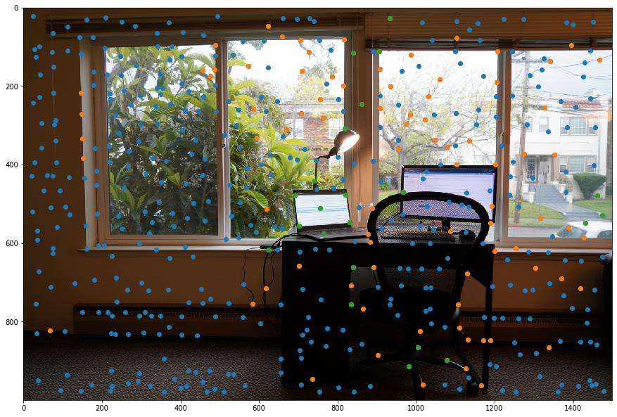
Harris Interest Point Detectors
The starting point for this paper is through the use of the Harris Interest Point Detectors. We can visualize what these points look like for the two apartment images.


Adaptive Non-Maximal Suppression
We can see that we have a lot of points that come out of the Harris Interest Point Detectors. We will then refine these points by using the adaptive non-maximal suppression algorithm described in the paper. The main idea here is that we would like to maintain strong descriptor corners / points, but we would also like them to be well distributed across the image. The results once again can be shown for the apartment images from above.


Feature Descriptor Extraction
Now we will have reduced the number of points, but we need to find correspondences between points. For this we will first extract feature desriptors (we do not do the more advanced rotation invariat parts described in the paper). With all of the feature descriptors extracted, we then move onto computing the SSD between each pairwise combination of the points. We throw away points which do not match or are not shared by using the a thresholded ration of the first nearest neighbor and the second nearest neighbor. Below we can see the following two images from before with the orange points now indicating those that are determined to be shared between the images.


RANSAC
We have made much progress from the initial points but we still see that there are quite a few of the orange points which do not seem to match. We thus turn to RANSAC for a robust computation of the homography matrix between the two points. I found that 10,000 or so iterations seemed to produce sufficient results and the computation was quite quick still. Below are the same two images with the ANMS points in blue, the feature points in orange, and then the points used to compute the final homography in green.

Results
Finally we can combine this with our algorithm from before which will allow us to automatically stitch images together. Below are the same three sets of images which we have been working with now stitched together totally automatically without any human input!
Apartment

City

Crater Lake