Image Warping and Mosaicing

Steven Cao / cs194-26-adx / Project 5 (Parts 1 and 2)

In this project, we'll see how to stitch images together into mosaics. This first part involves image stitching using manually picked point correspondences. In the second part, we will automatically find point correspondences.

Methods: Image Stitching

Image stitching involves three steps:

Take the pictures. The pictures should come from the same position but with the view rotated. Therefore, you should try to keep the camera lense fixed and only rotate it.
Pick points of correspondence. While 4 points are enough in theory, I collected 8 points to reduce noise.
Using these point correspondences, warp one image to the other such that the pairs of points lie on top of one another. The warp, which is a $3 \times 3$ matrix with $8$ degrees of freedom, can be computed with least squares as follows: $$ \begin{bmatrix} a & b & c \\ d & e & f \\ g & h & 1 \end{bmatrix} \begin{bmatrix} x \\ y \\ 1 \end{bmatrix} = \begin{bmatrix} w'x' \\ w'y' \\ w' \end{bmatrix} $$ Given this equation, we can first write $w'$ in terms of the other parameters. Then, we can solve for $a$ through $h$ by rearranging the equation as follows: $$ \begin{bmatrix} x & y & 1 & 0 & 0 & 0 & -xx' & -yx' \\ 0 & 0 & 0 &x & y & 1 & -xy' & -yy' \\ \end{bmatrix} \begin{bmatrix} a \\b\\c\\d\\e\\f\\g\\h \end{bmatrix} = \begin{bmatrix} x'\\y' \end{bmatrix} $$
Finally, once the first image is warped to the geometry of the second image, we can blend them together.

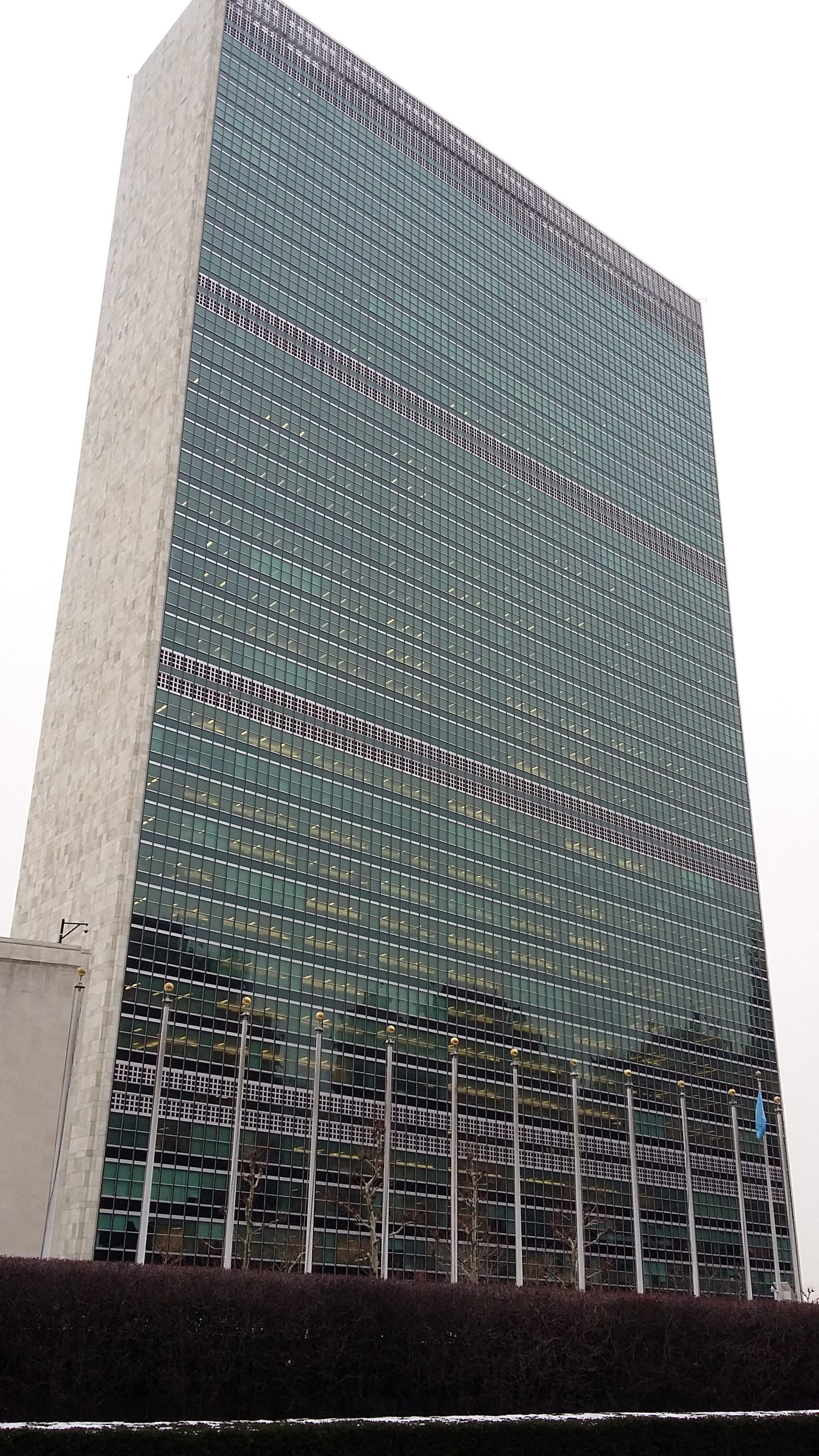
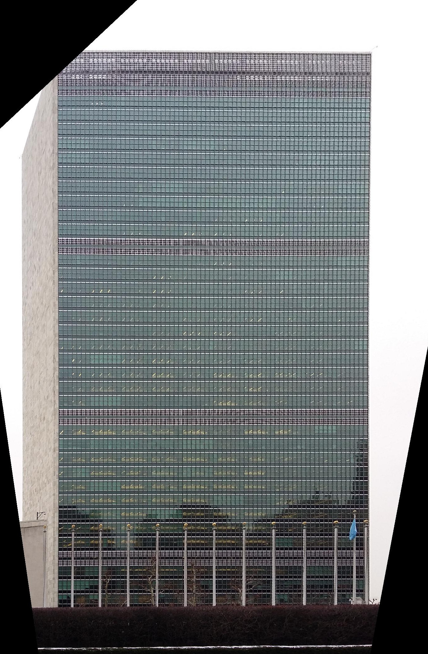
Results: Rectification

First, let's use warping for a different application, rectification. Rectification means transforming the image so that one of the planes is directly parallel with the image plane. We can perform rectification by (1) picking four points forming a square on the plane of interest, and then (2) warping these points into an actual square, or the points $(0,0), (a,0), (0,a), (a,a)$. Below are some examples. In the first case, we rectify to the right face of the building, and in the second case, we rectify to the face of the building.

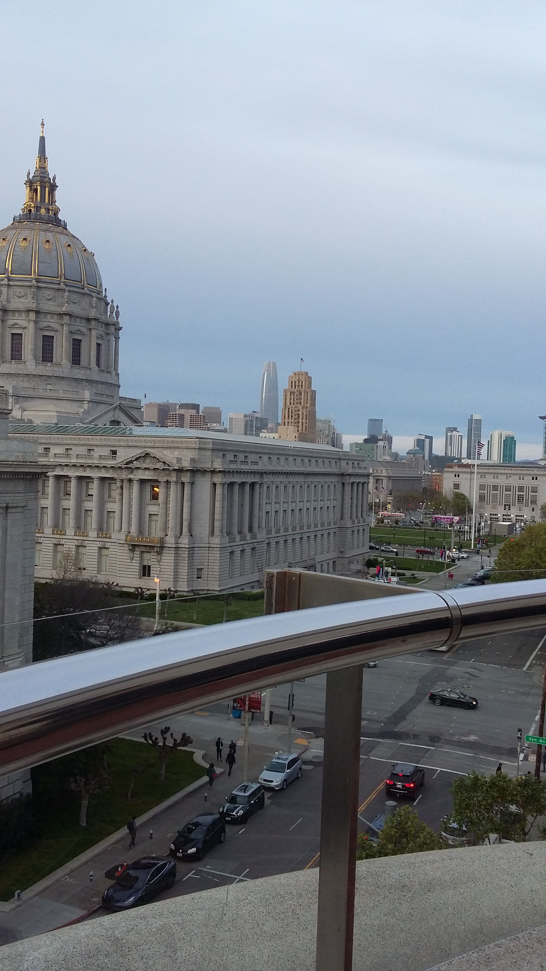
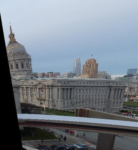
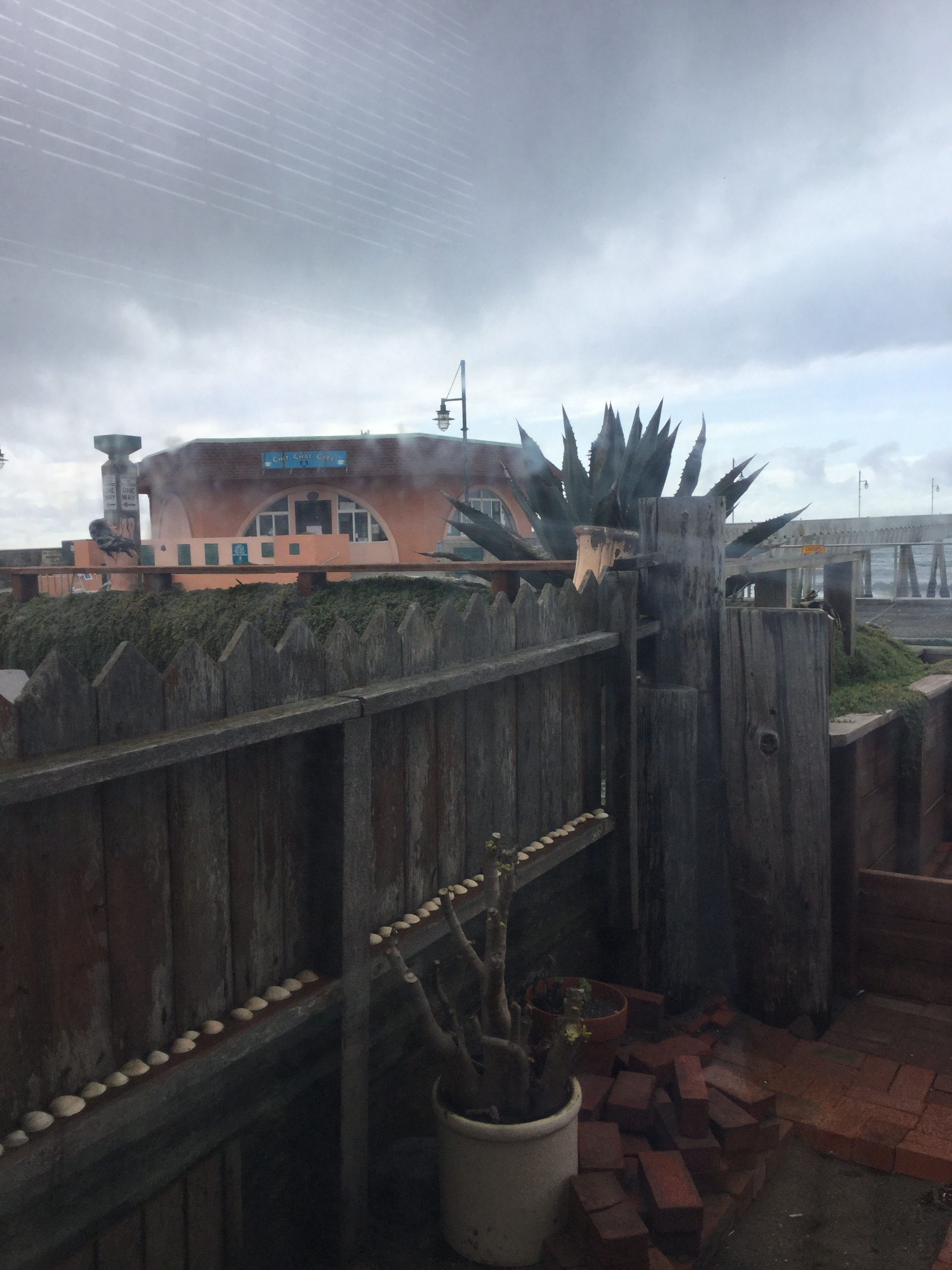
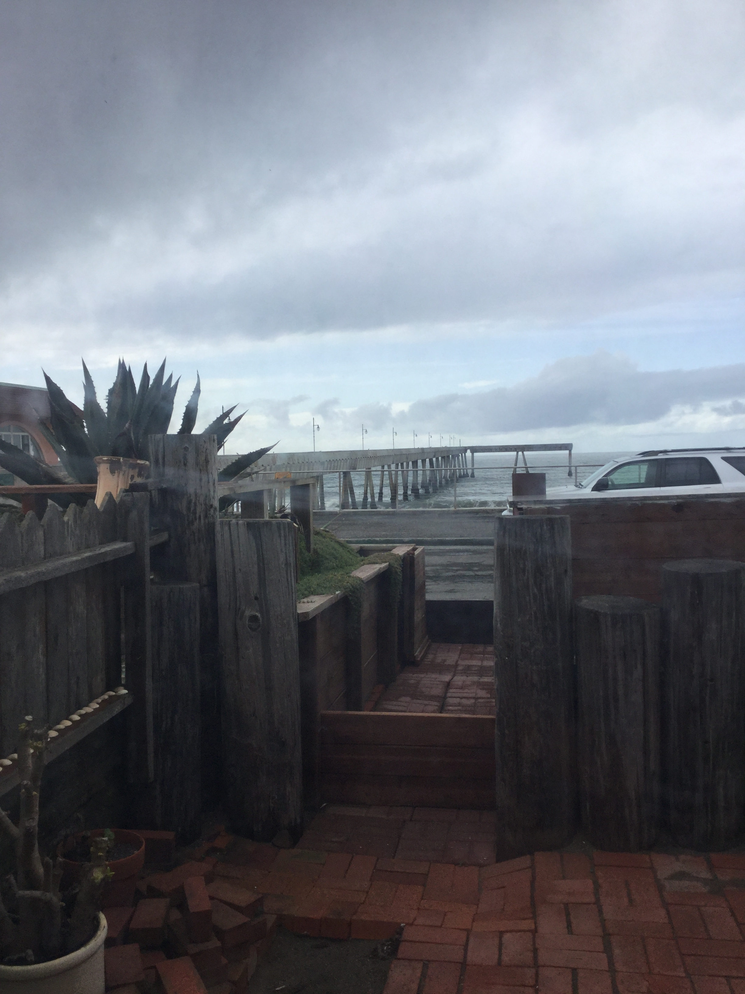
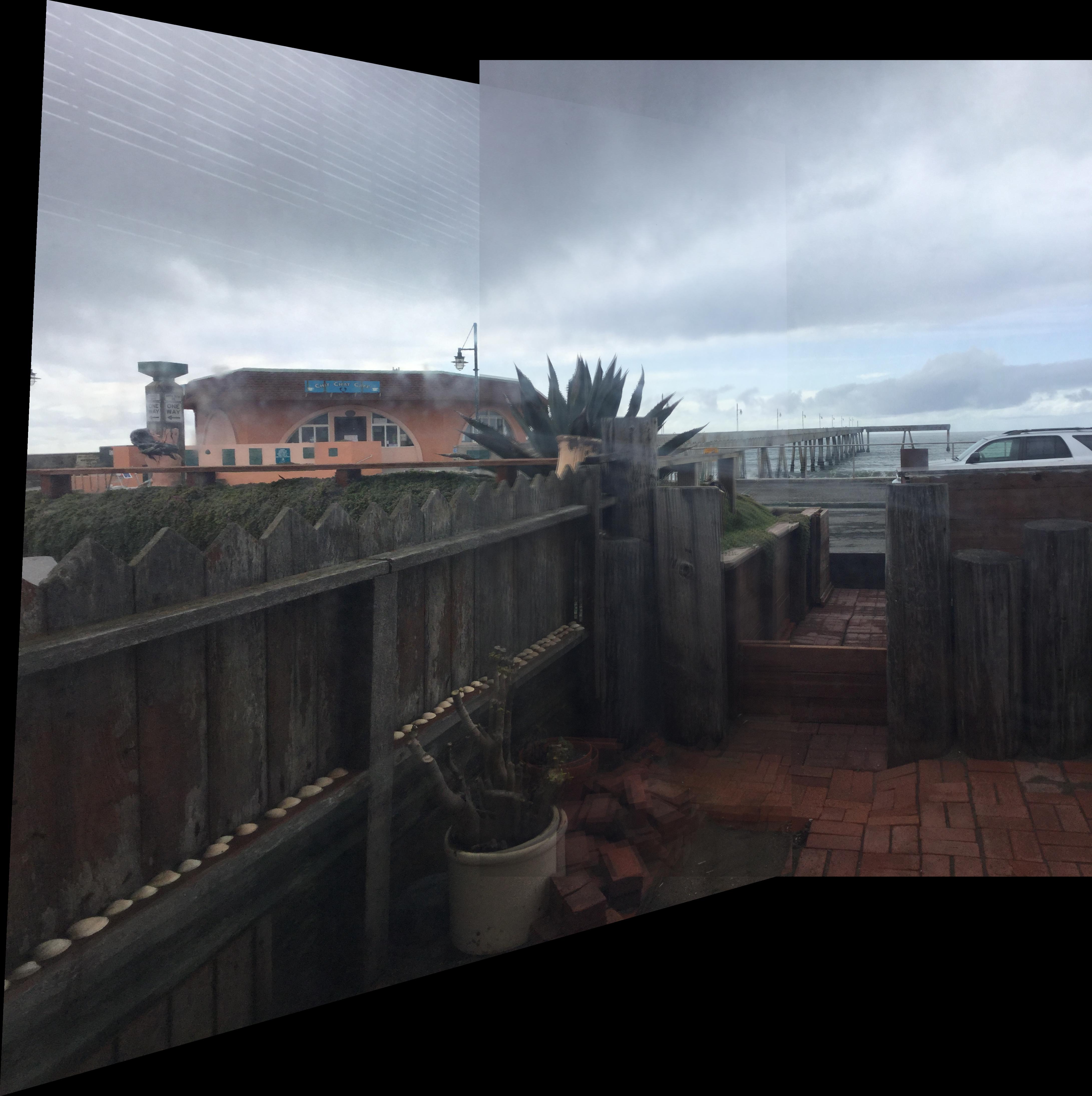
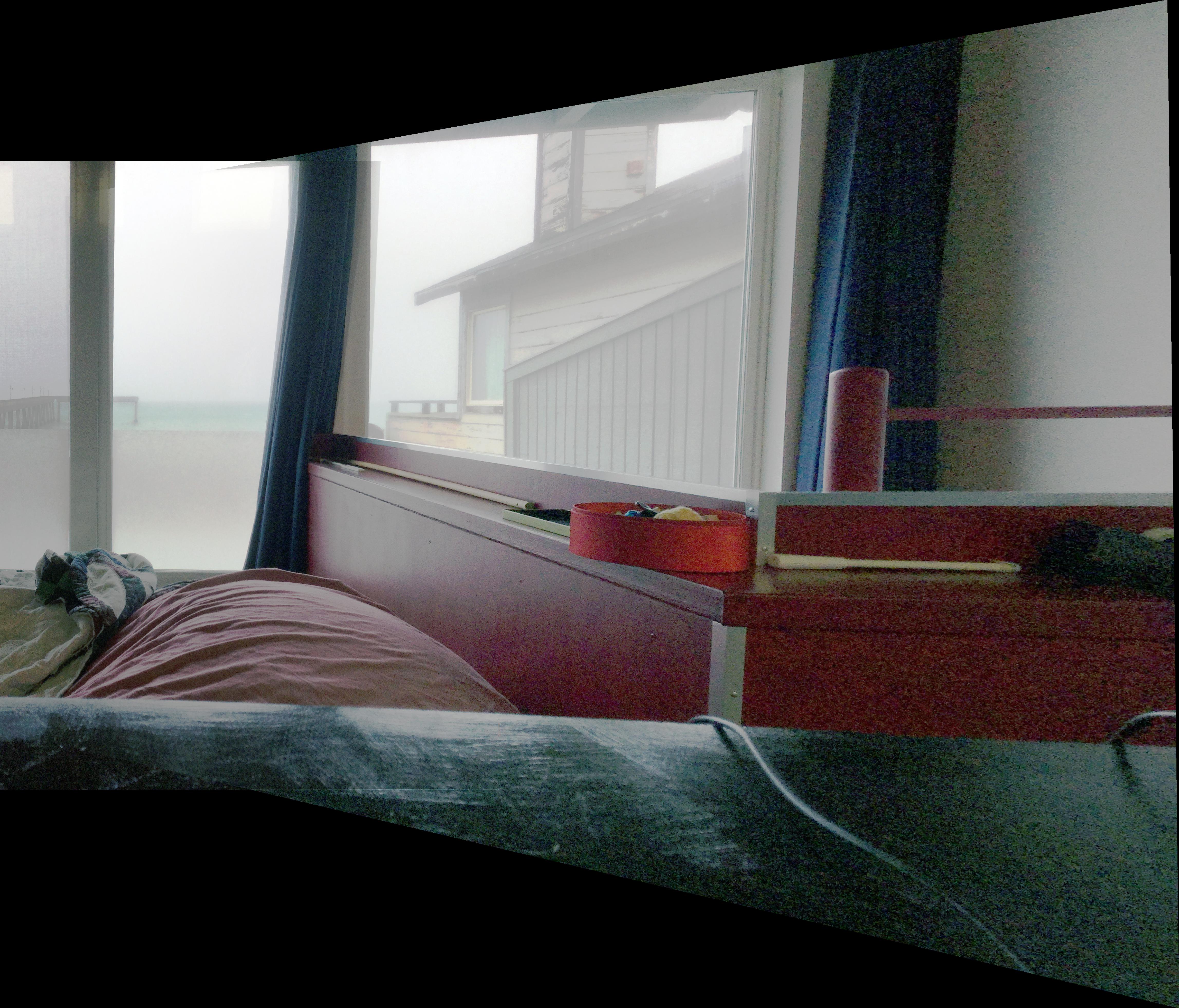
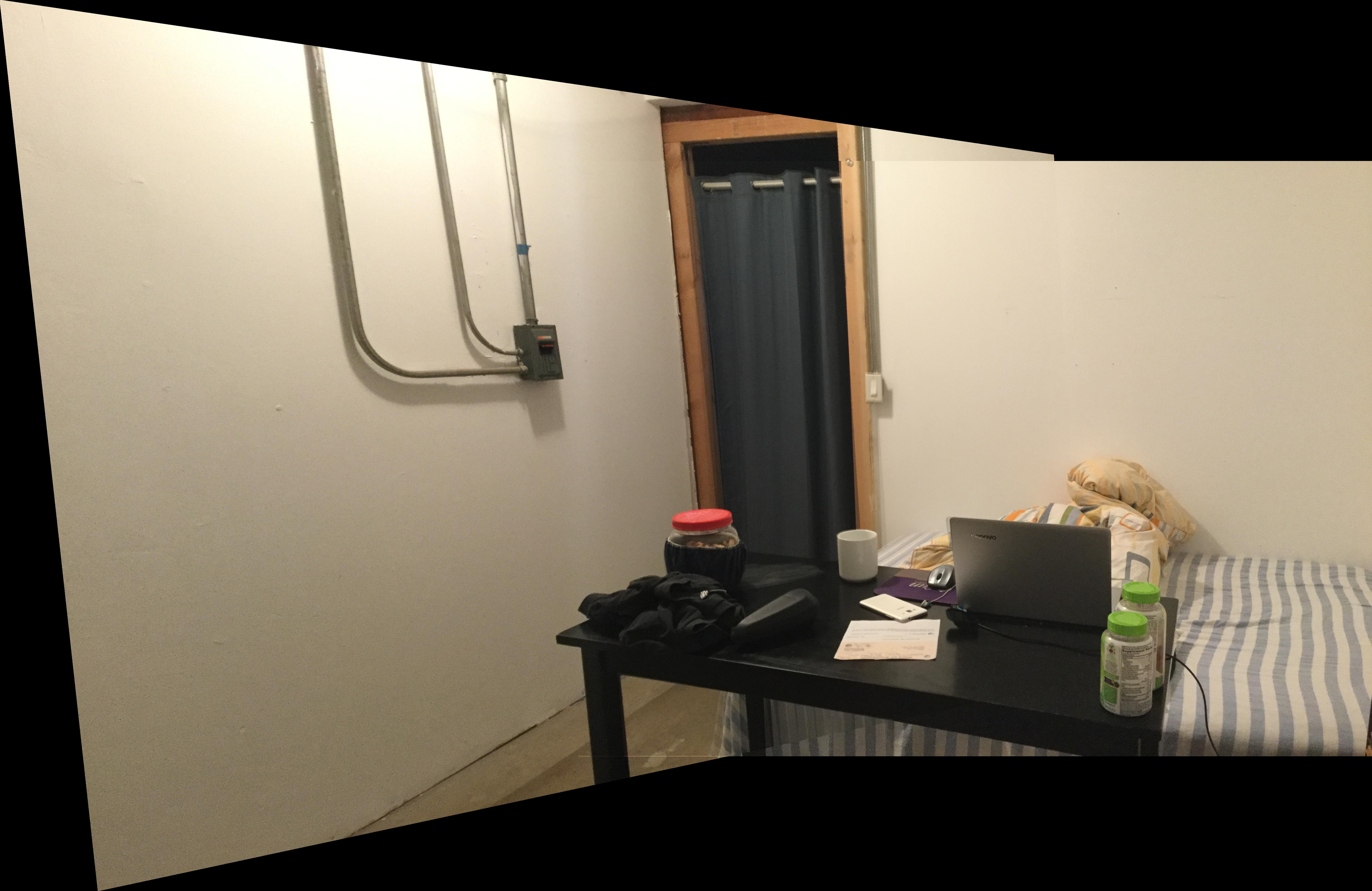
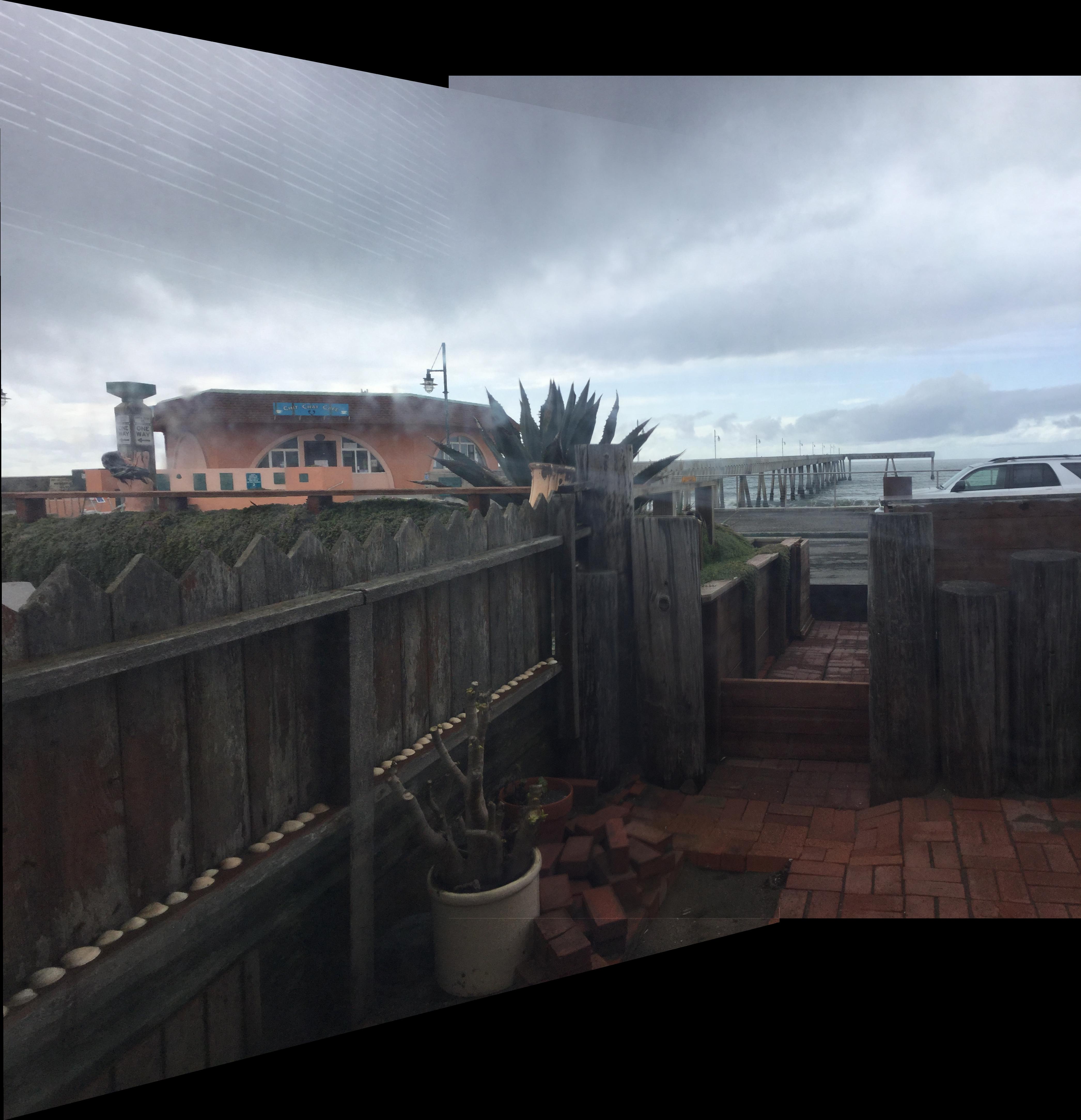
Results: Mosaicing

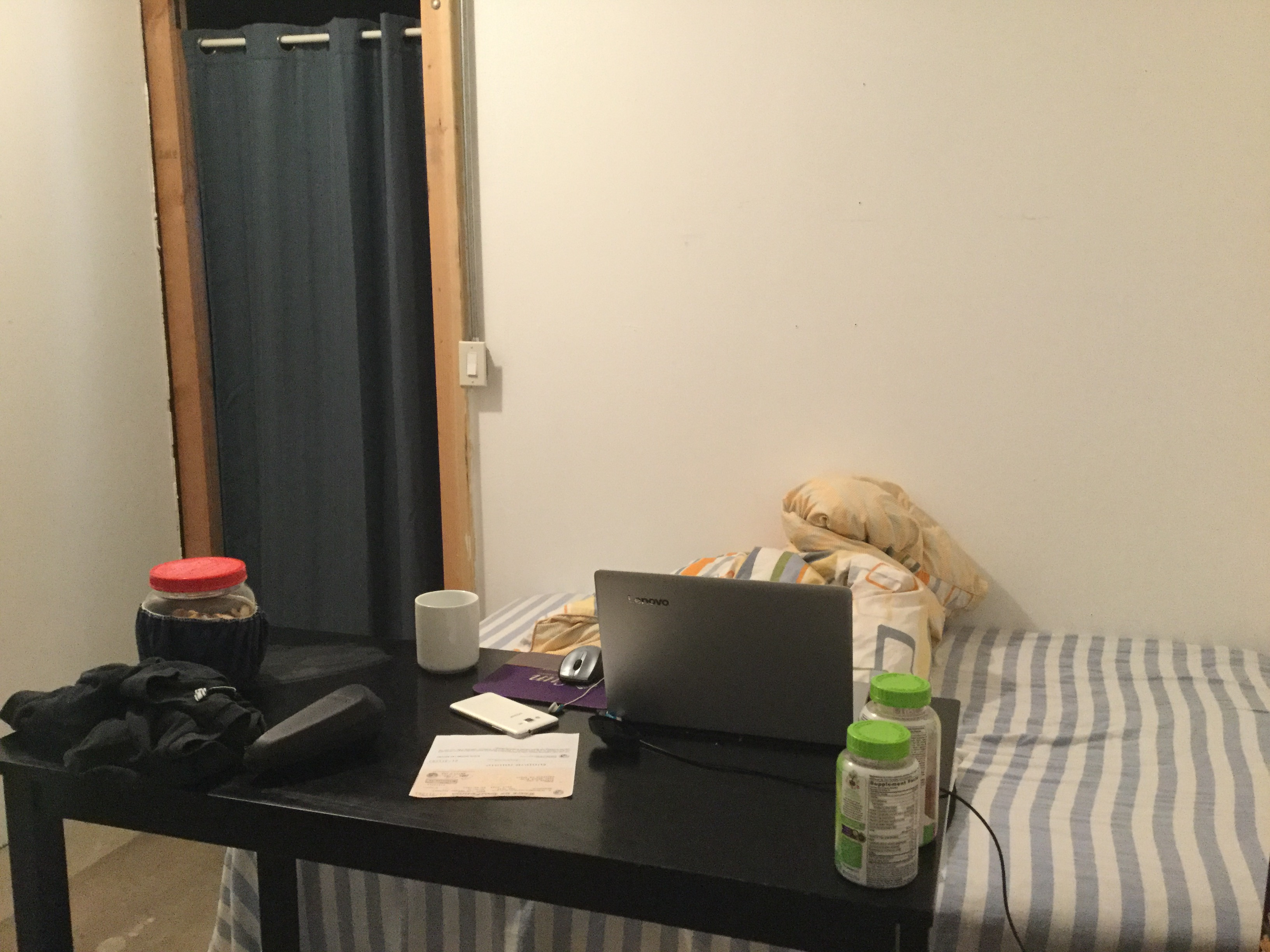
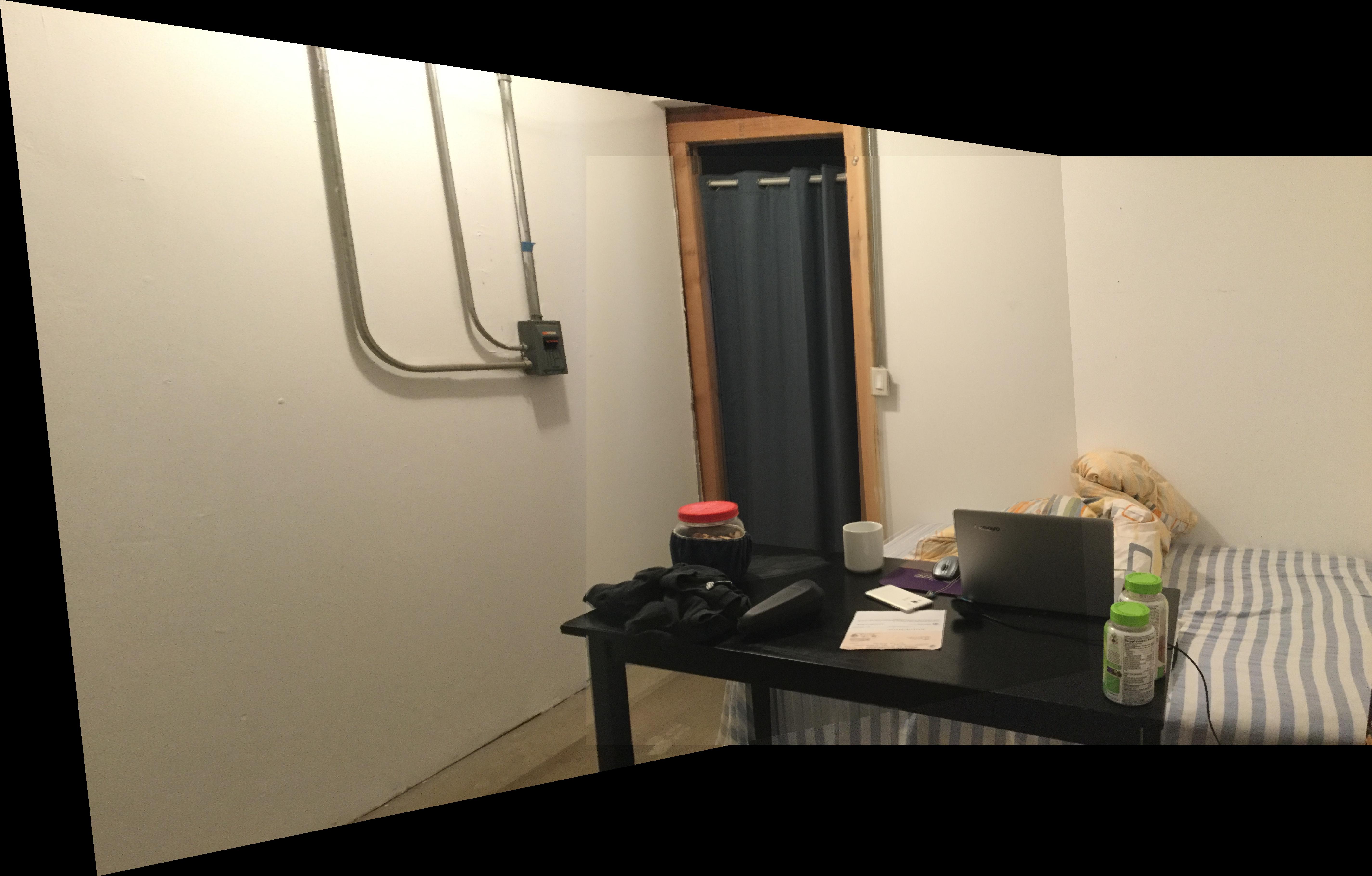
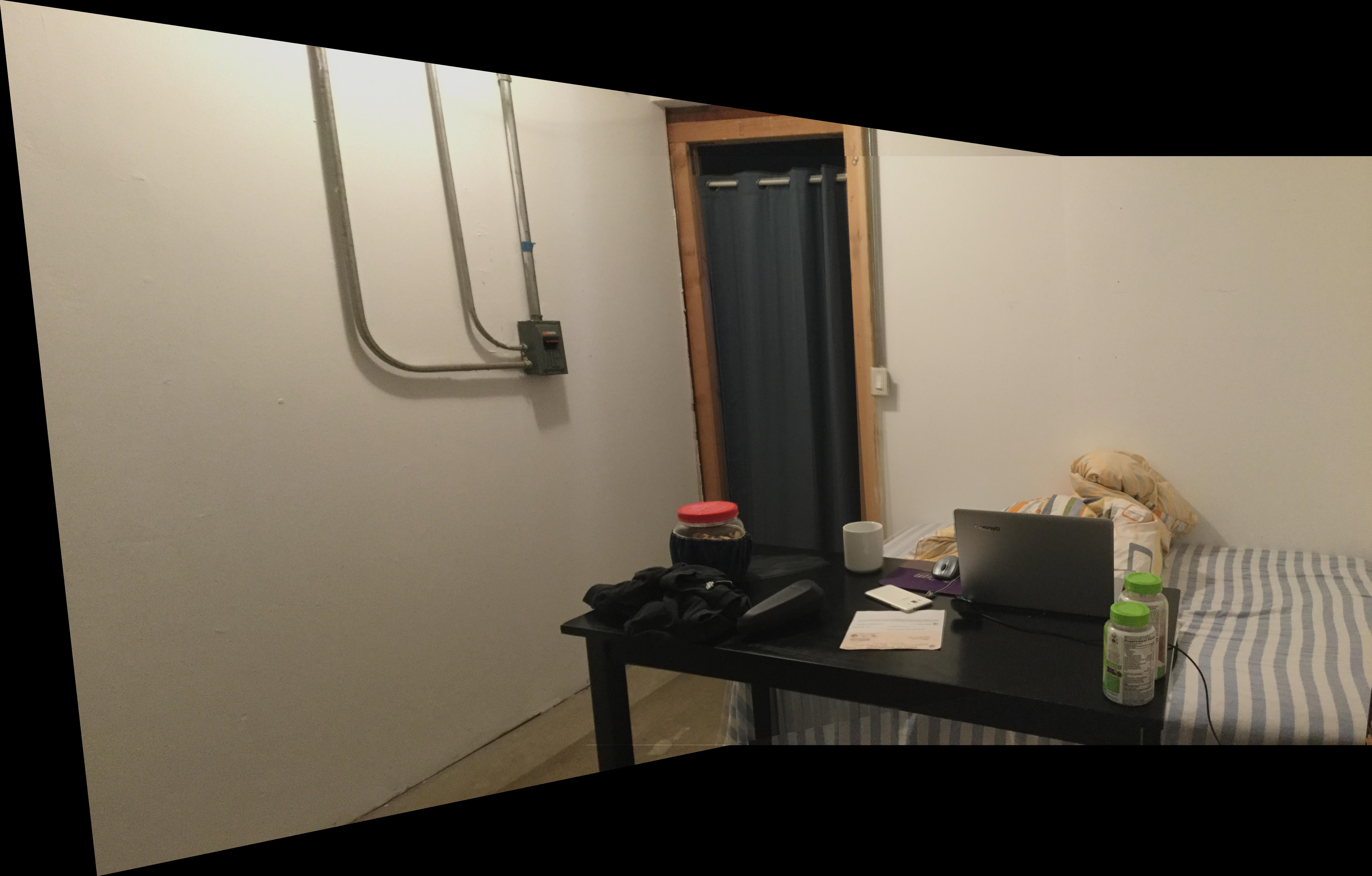
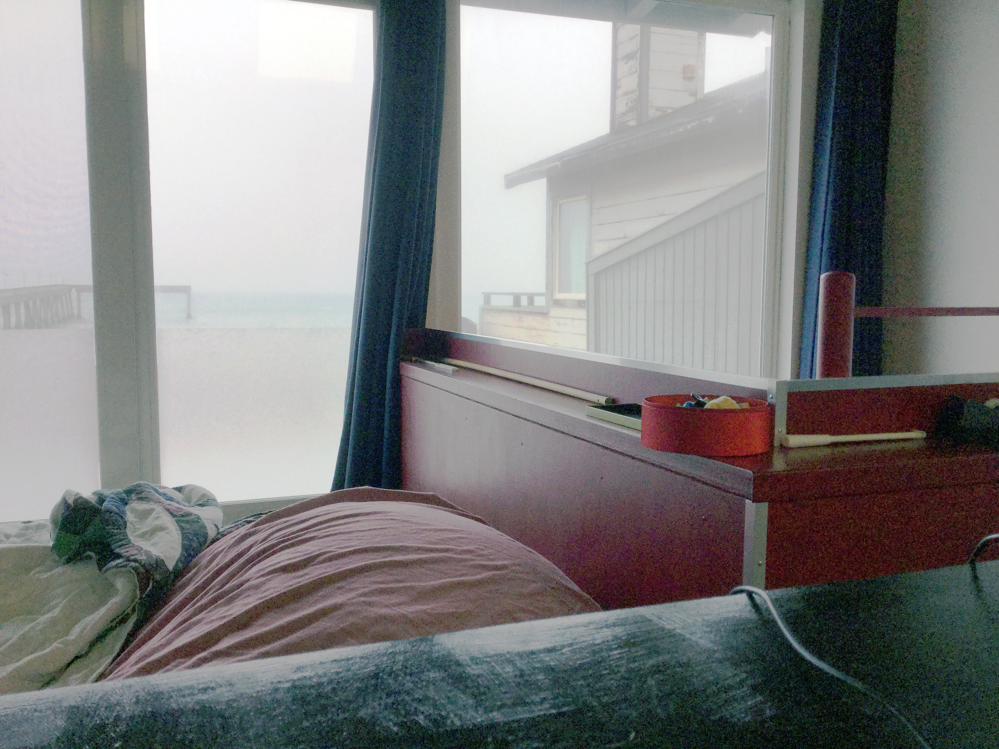
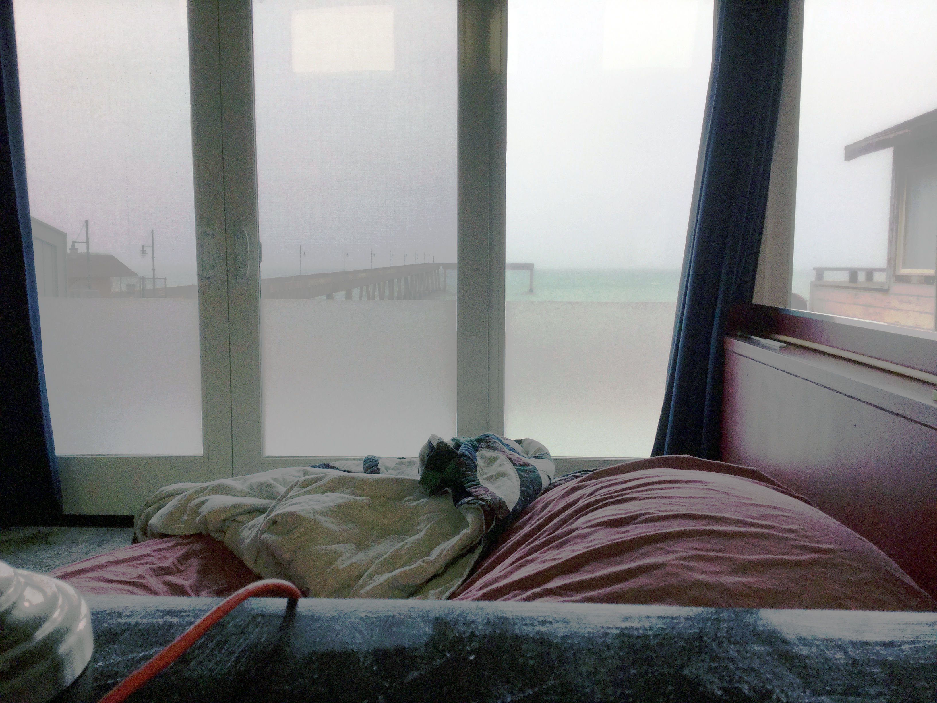
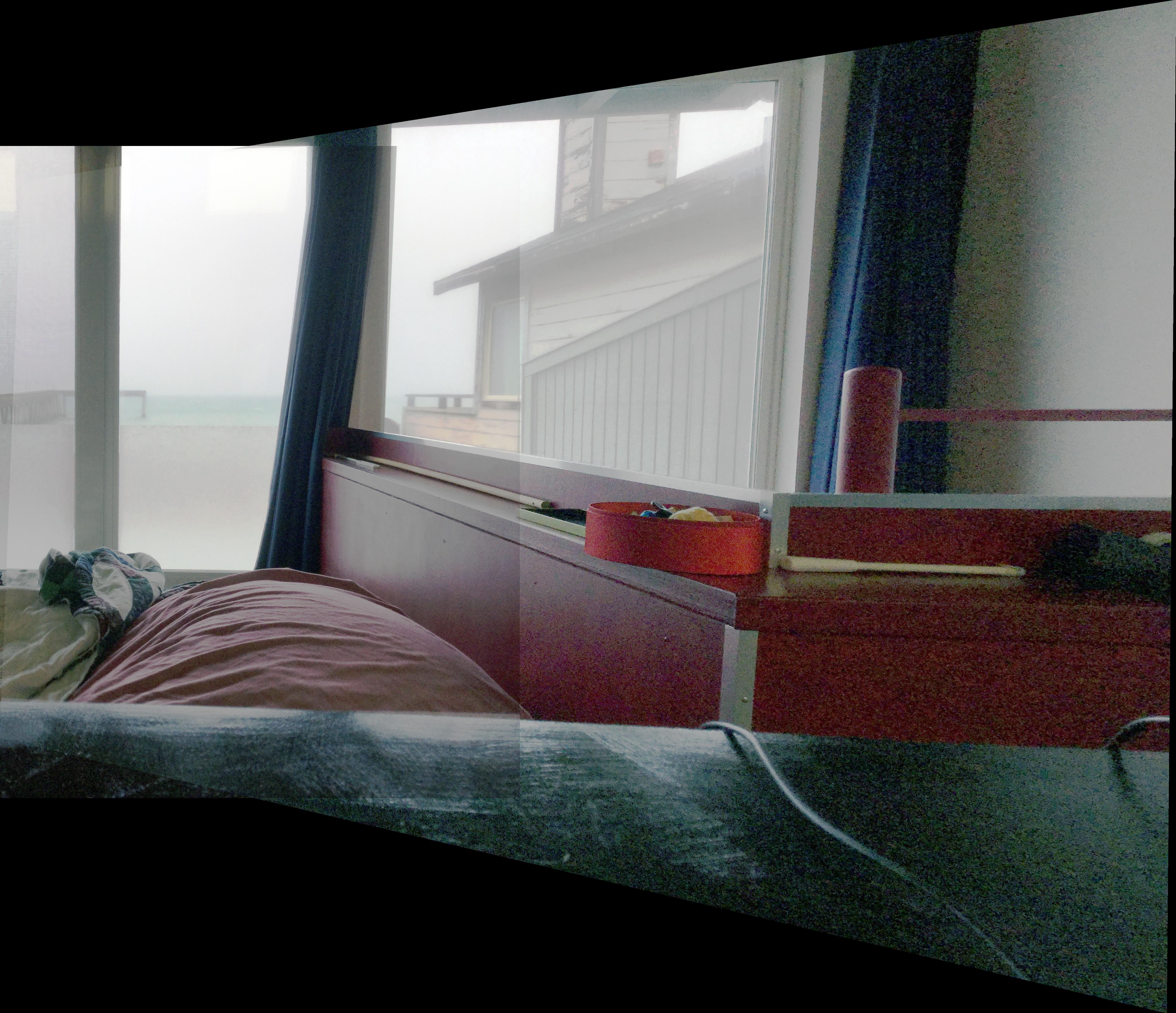
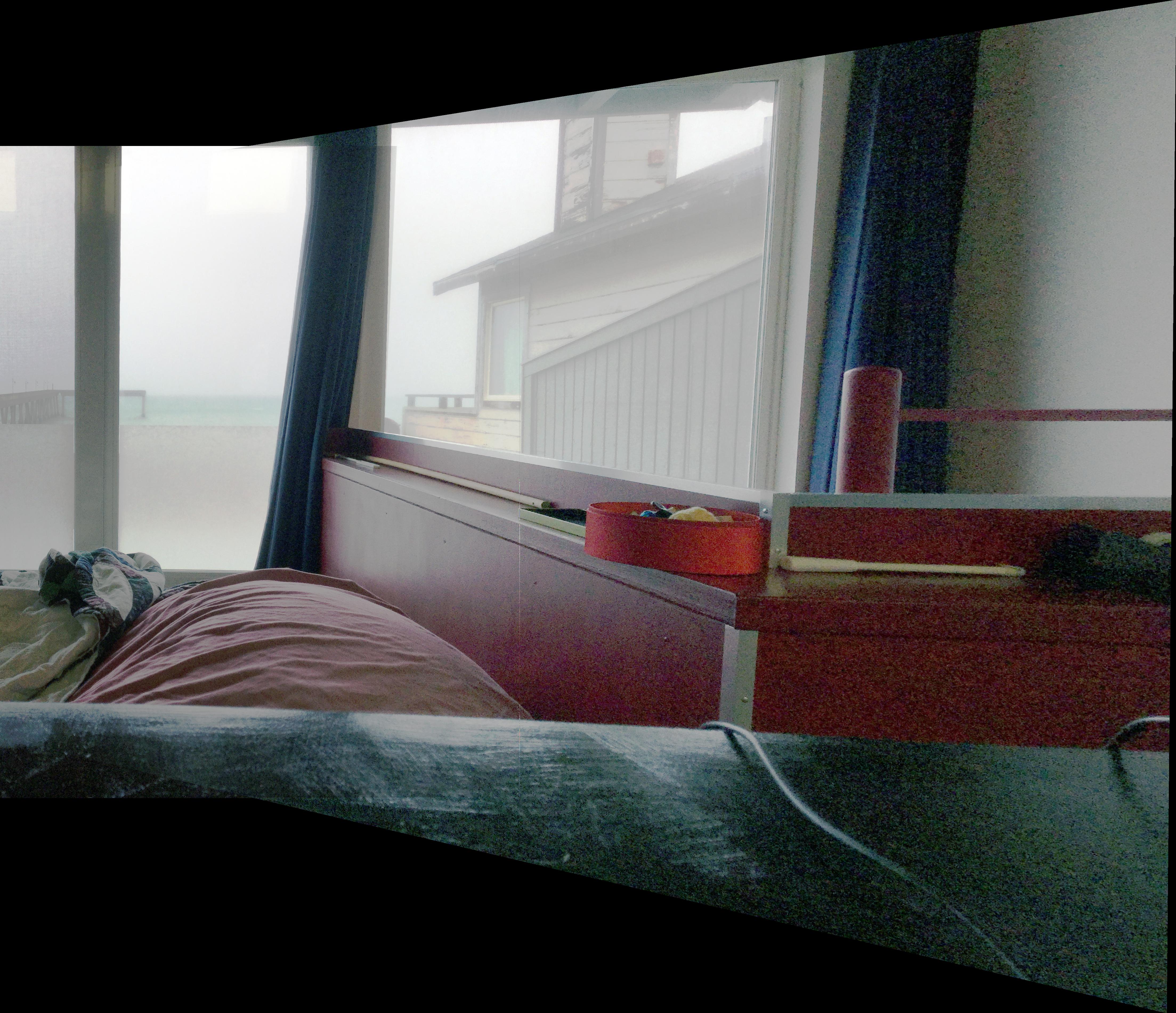
Next, let's look at examples of mosaicing. I took these pictures in my home. Unfortunately I couldn't get any nice pictures of scenery due to the quarantine. In each example, we show the two original images, the mosaic with simple average blending, and the mosaic with linear blending.

Methods: Automatic Point Matching

Image stitching requires us to manually pick points, which is tedious and prone to human error. What if we could find the point correspondences automatically? The following sections describe a series of steps to achieve this goal, following a simplified version of the approach described in Multi-Image Matching using Multi-Scale Oriented Patches.

Finding Candidate Points in Each Image: Harris Corners

First, we need to find candidate points of interest in each image. Intuitively, a point on a wall or some other low-detail region will not be useful for matching, while a corner will be good for matching because it is easily localized.

We will accomplish this goal by using Harris corners. At a high level, to get the score for a point in the image, we can take a window, wiggle it around, and look at how much the window changes as it moves. The amount of change will be small for a wall and large for a corner.

The actual Harris corner detector is a first-order approximation of this procedure. For more details, see here.

Finding Candidate Points in Each Image: Harris Corners

Once we have a ``corner score'' for each pixel in the image, we can take the local maxima of this corner score, giving us a set of points in the image.

The actual Harris corner detector is a first-order approximation of this procedure. For more details, see here.

Finding Candidate Points in Each Image: Adaptive Non-Maximal Suppression

Next, we will reduce the number of candidate points using a technique in the paper called Adaptive Non-Maximal Suppression. We want to keep the points with the highest Harris score, but we also want the points to be well-separated. To accomplish this goal, for each candidate point, let's define the suppression radius to be the following: $$ r_i = \min_j |x_i - x_j|\ \text{s.t.}\ h(x_i) \lt 0.9 * h(x_j) $$ In words, one point $x_j$ suppresses another point $x_i$ if its Harris score is much higher, or $h(x_i) \lt 0.9 * h(x_j)$. Then, the suppression radius is the distance to the closest suppressing point. Then, good points should have large suppression radii, which means that their Harris score is large compared to all other points in the neighborhood.

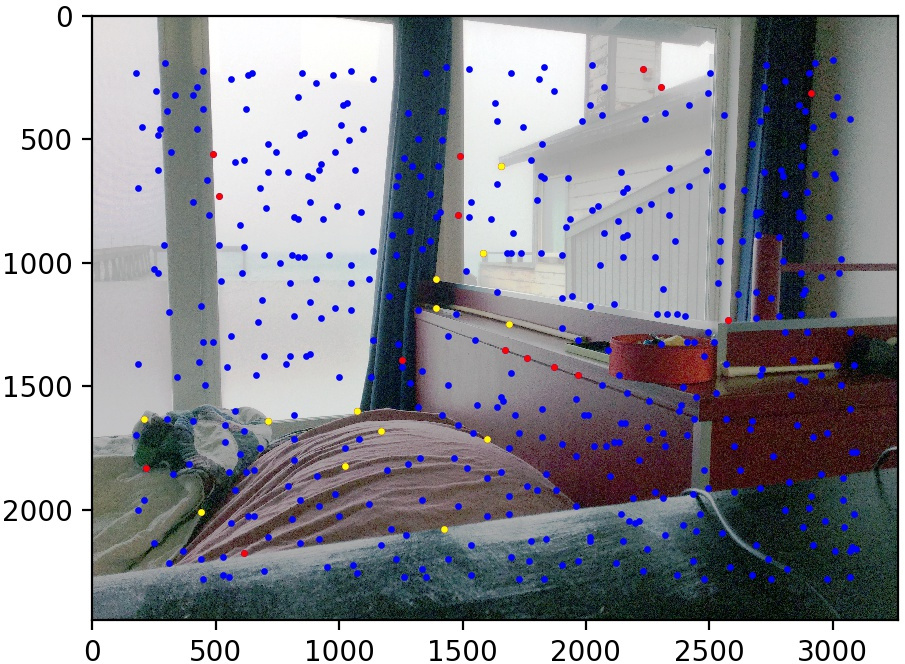
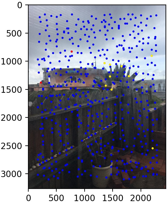
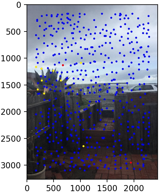
Given these radii, for each image, we will pick the $500$ points with largest radii. Examples are shown in the results section.

Matching Points: Feature Descriptors

Now that we have 500 points in the two images, our next goal is the find matched points between the two. Our approach will be to define a feature descriptor to describe each point. Then, we will define the distance between two candidate points to be the L2 distance between their feature descriptors, and we will take nearest neighbors to be matched points.

Our feature descriptor is very simple: first, we will take a 40x40 patch around the point. Then, we will blur by resizing this patch to 8x8. Finally, we will subtract the mean and divide by the standard deviation. This descriptor gives us a length-64 vector for each point.

Matching Points: Finding Nearest Neighbors

Unfortunately, simply choosing nearest neighbors leads to too many false positives. We will fix this problem by looking at the ratio between the first nearest neighbor and the second nearest neighbor. Then, we will keep points whose ratio is less than 0.3. Intuitively, if a point has two or more good matches in the other image, then it's likely that this point is generic and difficult to match. Therefore, we will pick points that have a very good first nearest neighbor but a bad second nearest neighbor, making it clear that these two points are in correspondence.

After performing matching, we are left with about 10 point correspondences. Examples are shown in the results section.

Computing the Homography with RANSAC

Even with the above procedure, we will still have a few outliers that will completely ruin the homography calculation. To find and discard outliers, we will use RANSAC, which performs the following steps:

Select 4 points at random and compute the homography from them.
Find the inliers, or point pairs whose distance $ \| x_1 - H x_2 \| < \epsilon$. We choose $\epsilon = 10$ for an image that is roughly $2000 \times 2000$.
Repeat the above two steps multiple times, and keep the inlier set that is the largest. We perform $50$ repititions.
Finally, fit the homography on just these inliers, and discard the rest of the points as outliers.

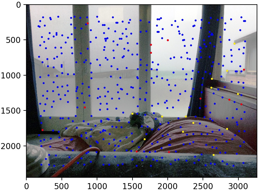
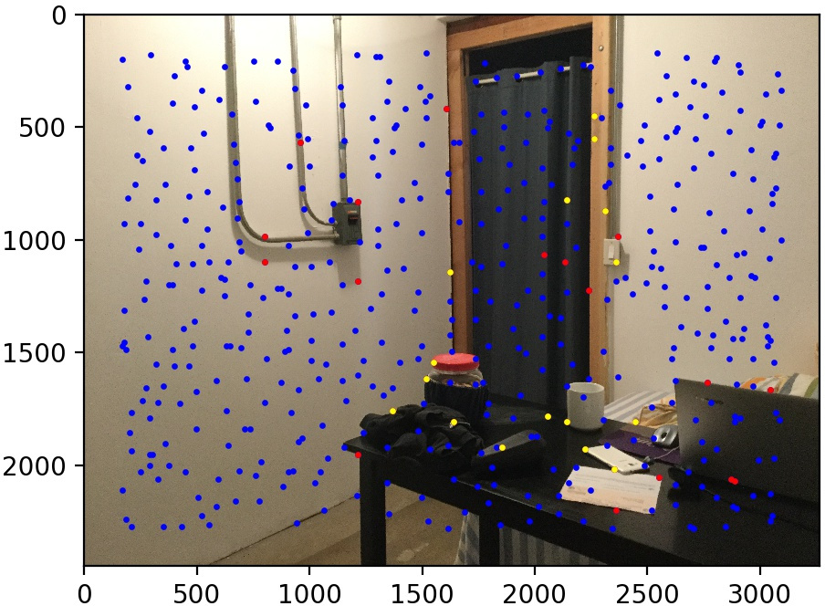
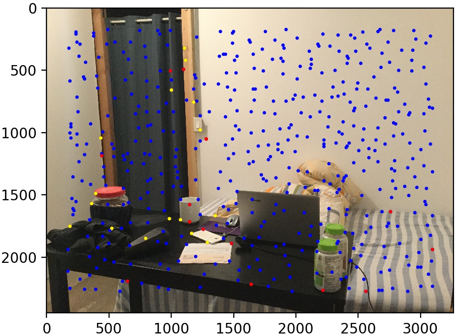
Results: Automatic Image Stitching

Let's look at some results of this procedure. We use the same three image pairs as in the manual case. We also show the points found by Harris corner detection and Adaptive Non-Maximal Suppression (in blue), the matched points that are outliers (in red), and the matched points kept by RANSAC (in yellow). The method performs quite well!

Conclusion

I enjoyed making mosaics and I am glad that I now have this technique in my toolkit. It was interesting to learn that you actually shouldn't move the camera while taking the panoramic photo. It seems that since most people take pictures of scenery, which is faraway, the parallax effect is less noticable. But during the project, I realized that it matters a lot if you take pictures of nearby things! It was also very cool to see how well the automatic point-finding algorithm worked.