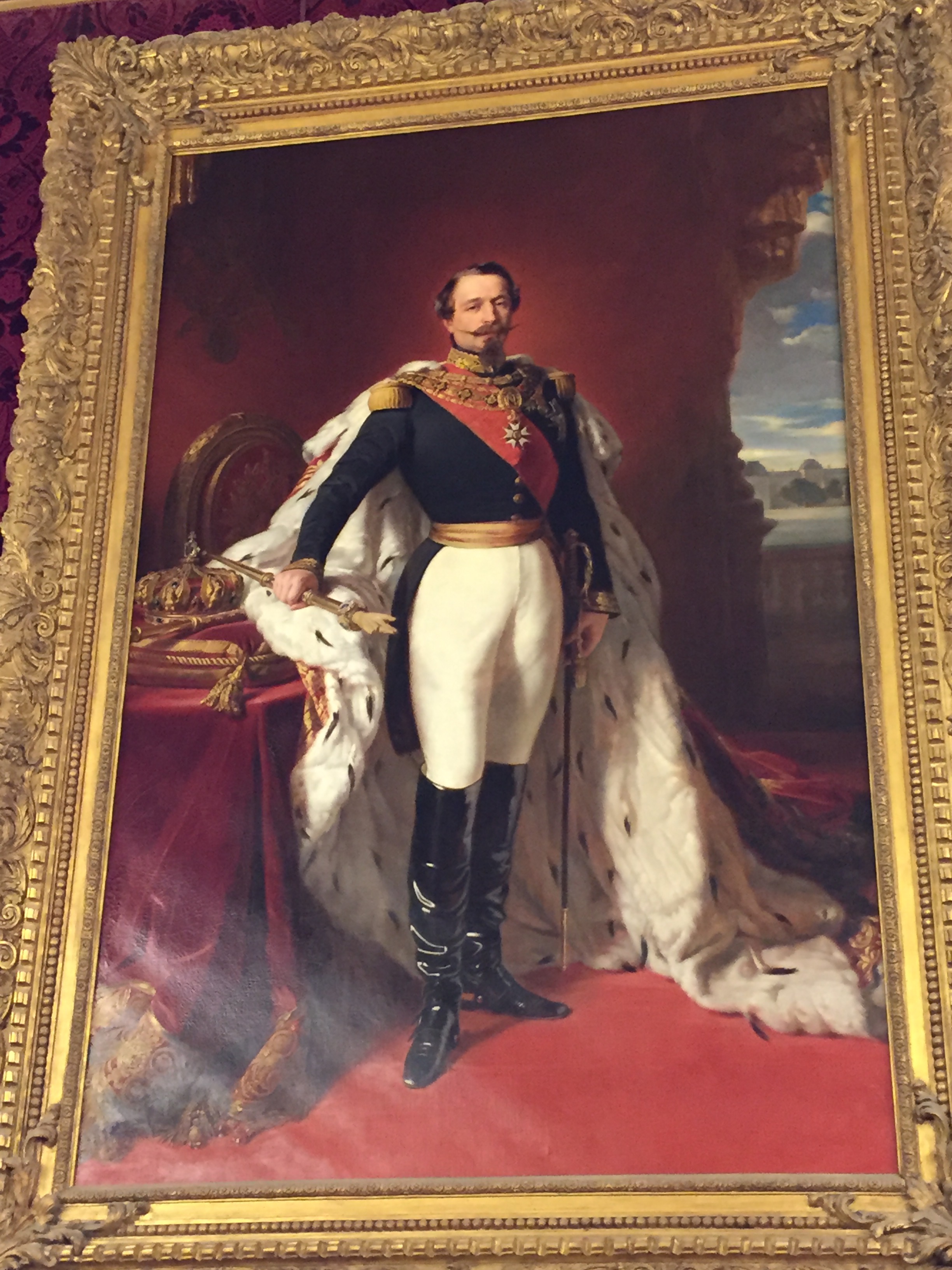
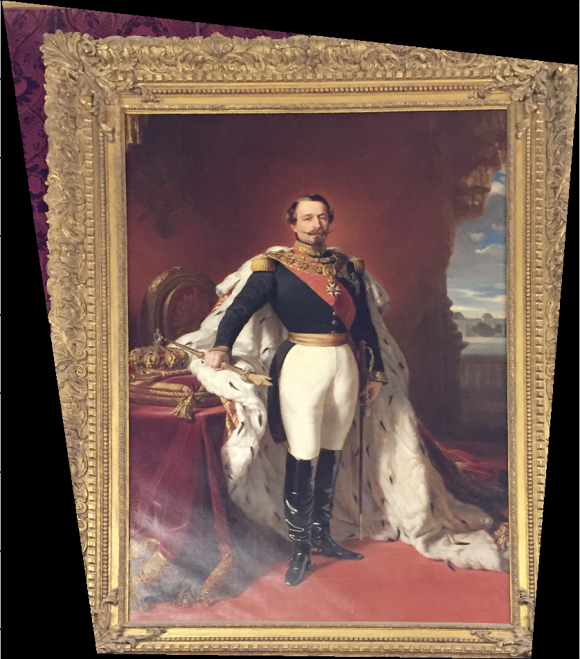
After finding an image that I wanted to rectify (am image of Emperor Napoleon III that I took in the Louvre), I selected four points at the corners of the painting. Then I defined four points of a rectangle that I wanted to rectify the painting onto. Using these four points, I could apply least squares in order to solve for the homography matrix H which converted between the two coordinate systems.
Next, I took the four corners of the original image and applied H in order to find the destination coordinates. Using these, I found the size of the target image.
After that, I used skimage.draw.polygon to iteratively list all of the coordinates in the target image. I used the original four points, but this time swapped the order of the coordinates in order to find the inverse homography matrix H_inv. Using this H_inv matrix, I found the point in the original image which corresponded to each point in the target image (oftentimes they did not exist, so I had to filter out the points which were outside of the range of the original image). Finally, I assigned the pixel value at that point in the original image to the corresponding point in the target image. Once all of the points were processed, I had my rectified image!
The most important thing that I learned was how to combine many corresponding points into a single transformation using least squares.
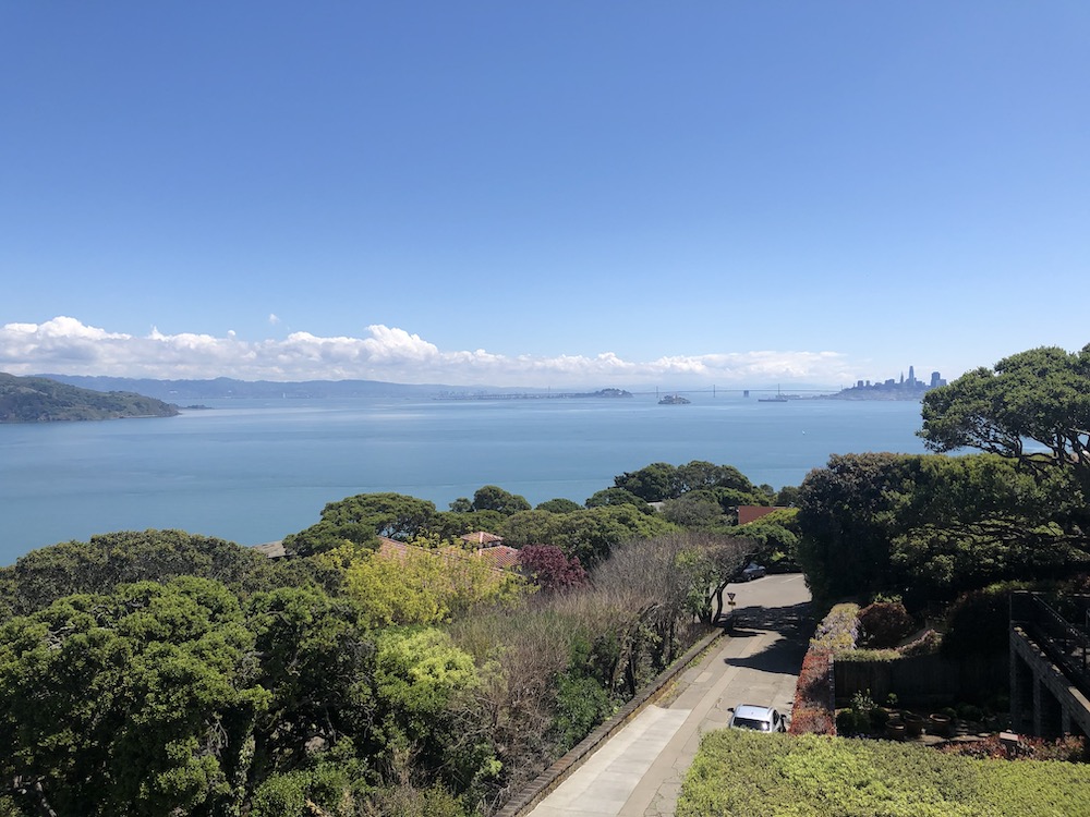
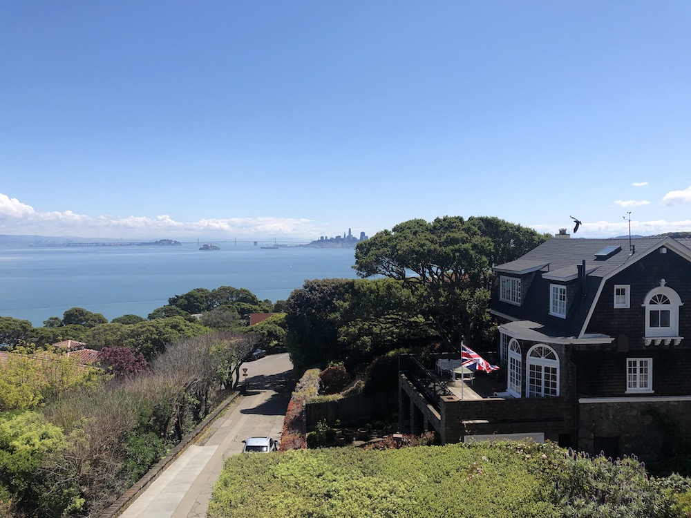
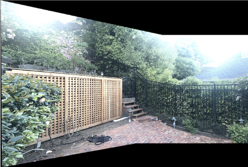
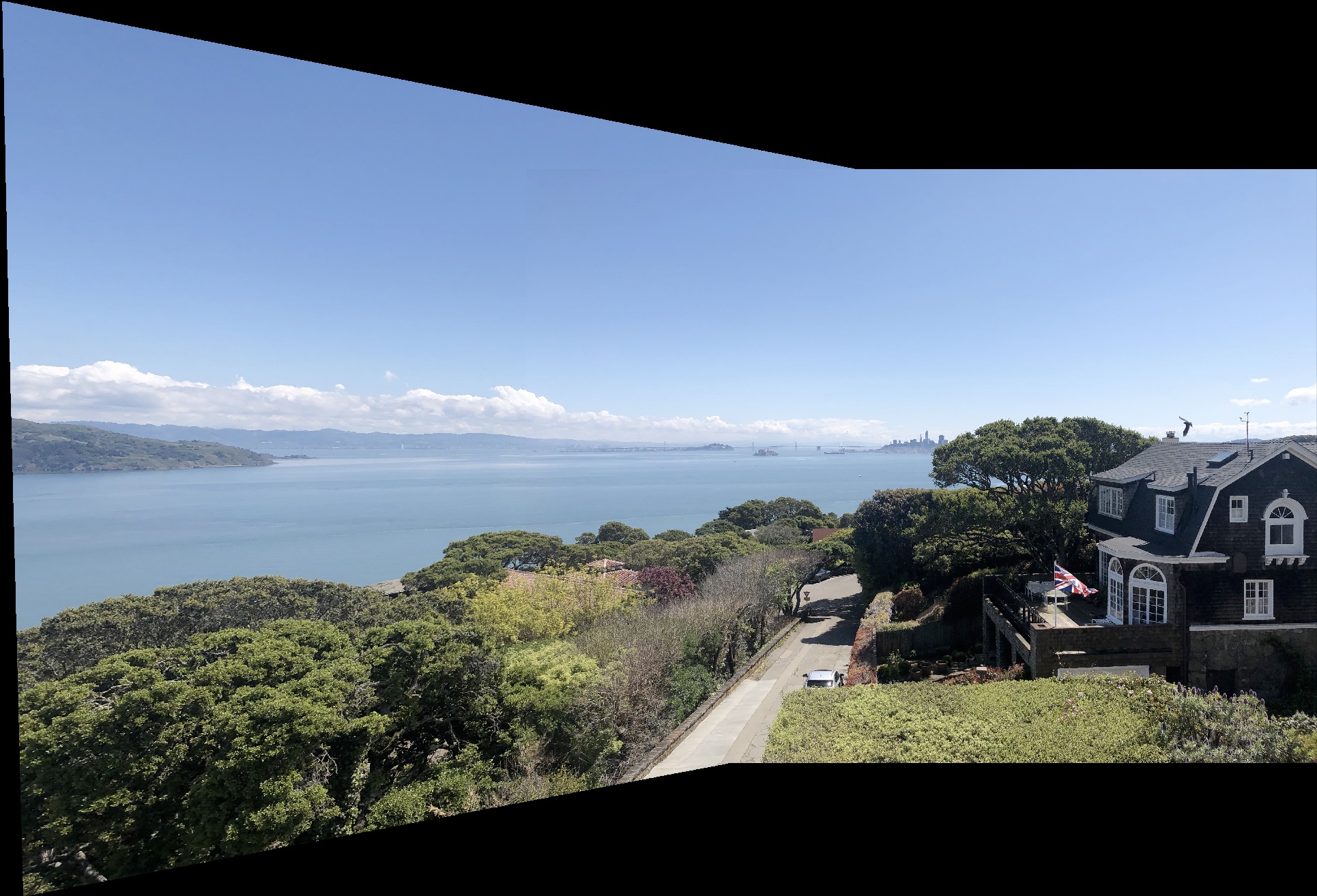
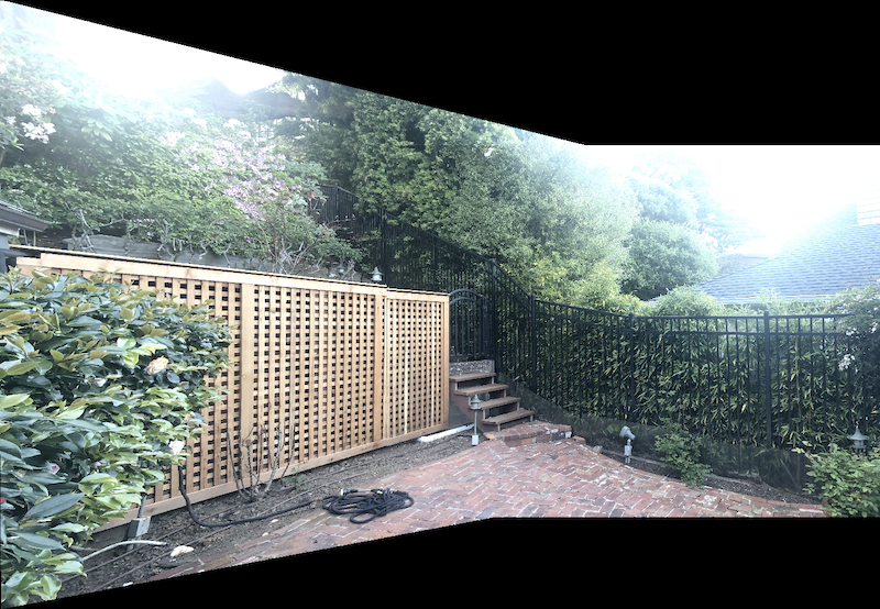
Once I had the ability to warp images based on homography, I could attempt to combine two images into a larger unified image. I took two images of the San Francisco Bay from my balcony, each only differing by a rotation of about 30 degrees. I specified eight corresponding points in both images on recognizable landmarks: Alcatraz Island, the bay bridge, parts of the SF skyline, etc. Then I computed the homography from the left image to the right (H) and the right to the left (H_inv). I chose to warp the left image into the perspective of the second.
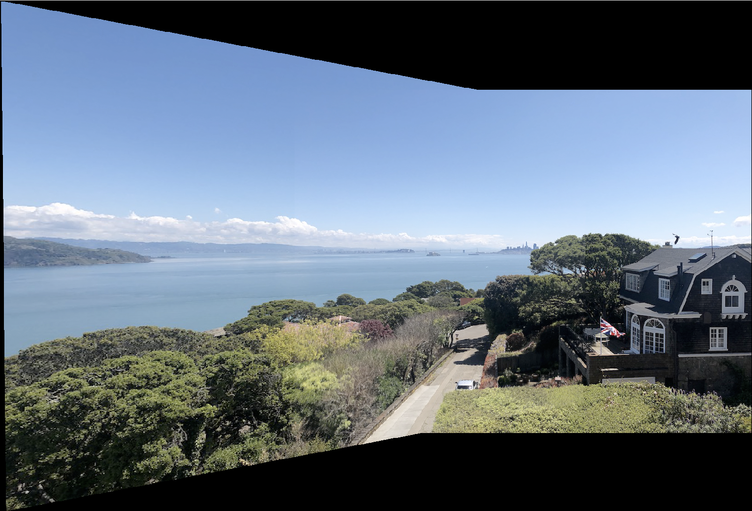
Using H, I warped the corners of the left image into the perspective of the second. Then I found the size of the target image by taking the extremes of the transformed corners and the original right image corners.
In order to populate the target image, I created a polygon using skimage.draw.polygon and the four transformed corners of the left image. I applied H_inv to the coordinates yielded by this function, and assigned the pixel values of all of the original coordinates in the target image to the pixel values at their corresponding coordinates in the left image yielded by H_inv. After this was done, I had finished mapping the left image onto the target canvas
Next, I mapped the right image onto the target image. This was quite simple, as the matching coordinates between them only differed by a constant translation (the translation is due to the fact that the left edge of the right image maps to somewhere in the middle of the target image, as the left edge of the target image needs to map to approximately the left edge of the right image). Since there were conflicting pixels here that were already populated by the left image, I assigned each pixel to the max of the right image pixel and the preexisting pixel value.
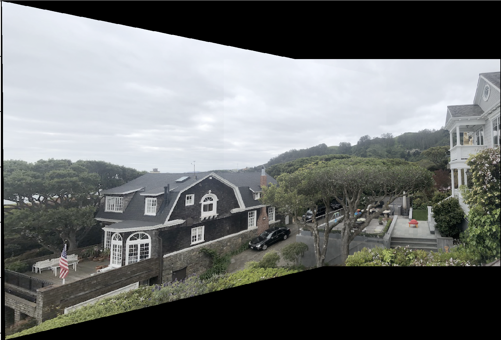
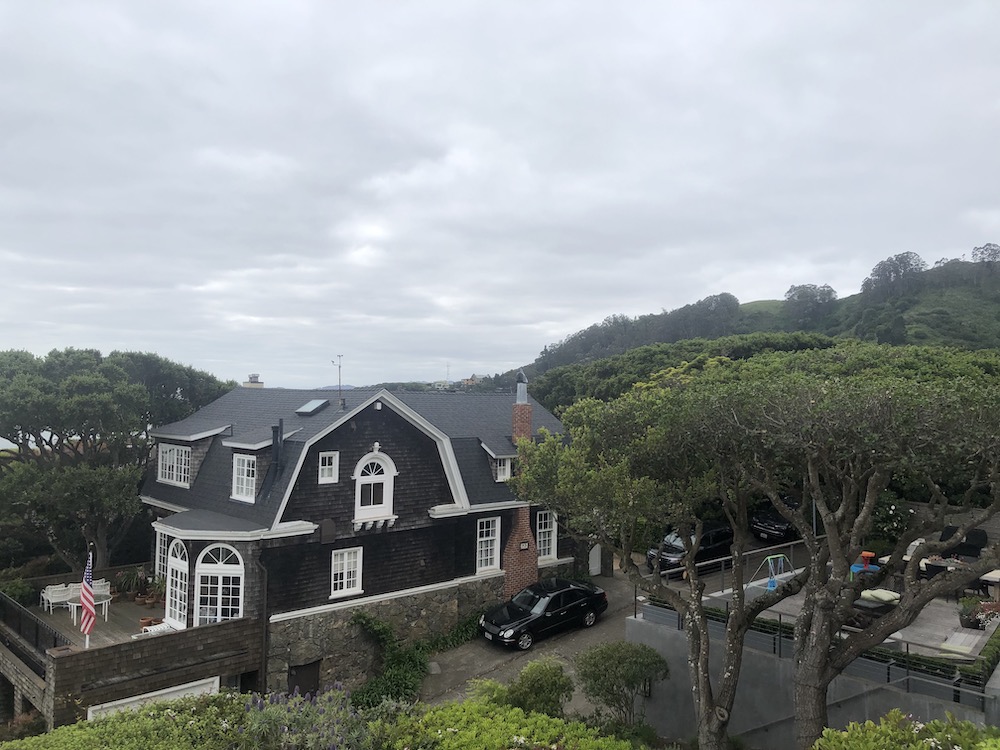
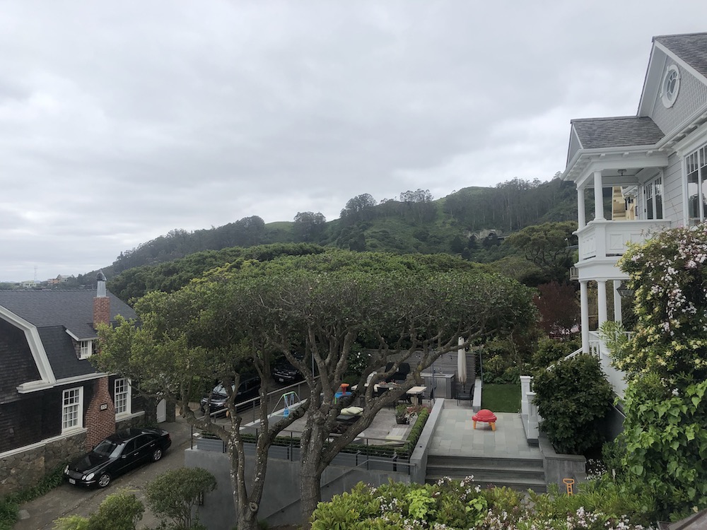
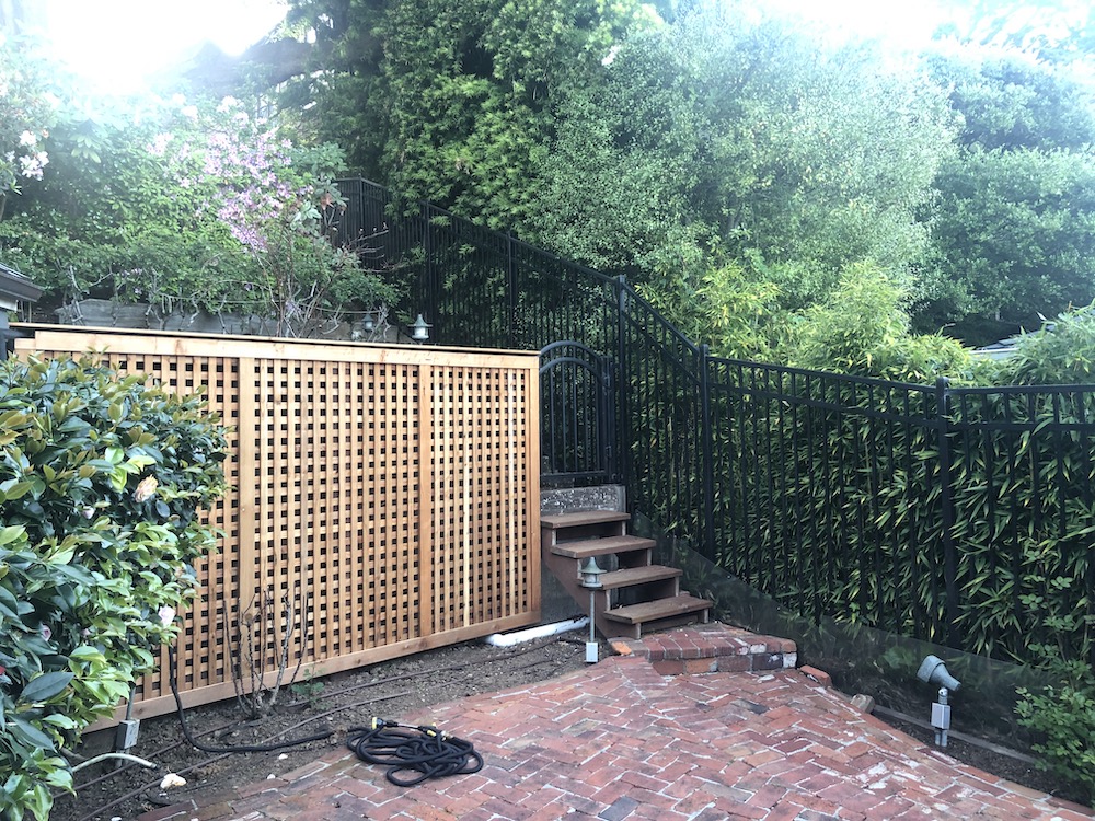
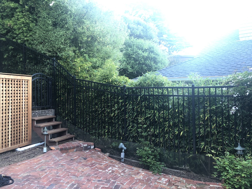
Here are some more examples:

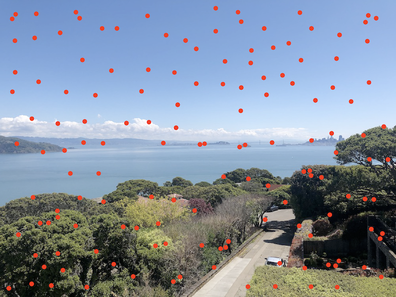
I began by running the provided Harris interest point detector. The following picture is an example of some of the points that it chose. For the final implementation, I used a minimum distance of one and didn't exclude any points from the ANMS procedure, however, this mean that superimposing the points on the picture left the picture entirely red. So for this picture, I used a minimum distance of 30. It is merely for illustration purposes.
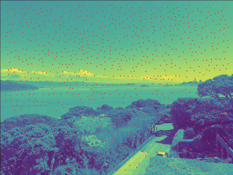
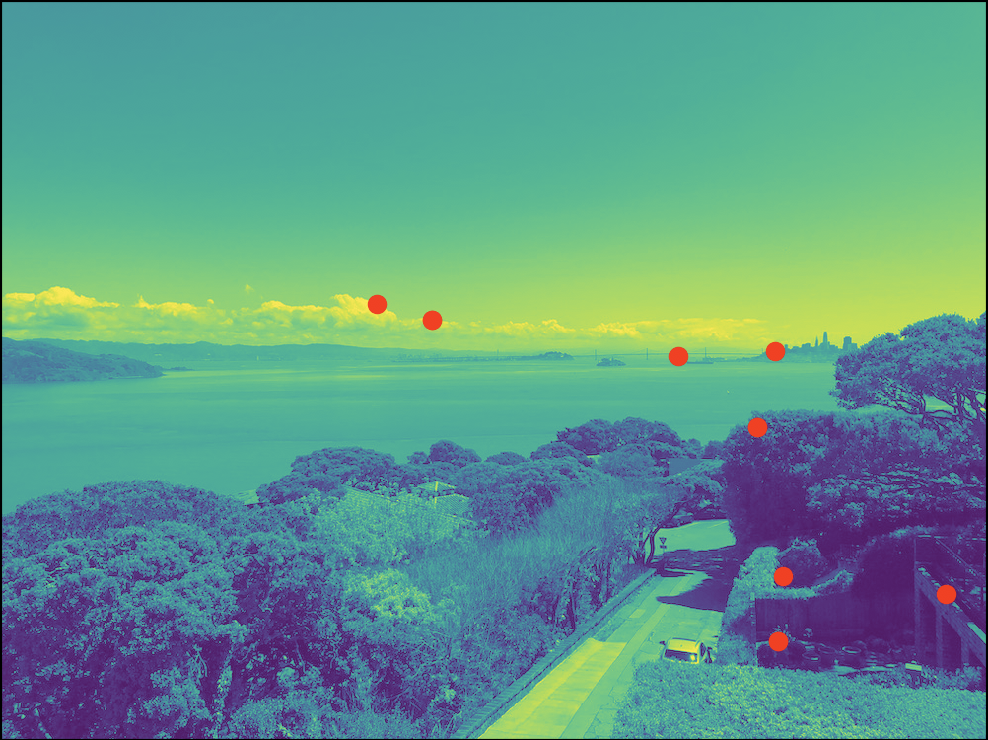
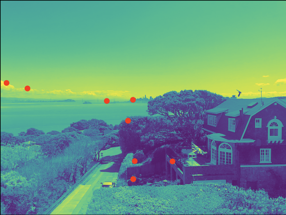
After that, I ran the ANMS algorithm given in the paper. First I used the provided dist2 function to get the distances between every pair of points. Then, for every row (corresponding to a point and its distances between all other points), I eliminated the columns corresponding to the points with weaker strengths than the point corresponding to the row. Finally, I took the min distance still remaining in the row. This gave the radius for each point. Then I sorted by min distance and chose the top 500 points. For illustration purposes, I displayed the top 100 points in the following photo:
We can see it matches neatly on things like the edge of clouds, parts of rooftops, the city skyline, etc. There are points in the sky, but I believe that this is merely due to the ANMS procedure which motivates evenly distributed points (i.e. the points in the sky are relatively weak).
After extracting the 8x8 patches (with zero mean and a standard deviation of 1, also these were subsampled by a 40x40 patch originally) around each of the points, I ran the feature matching process. This used the dist2 funct on the flattened patch vectors for each image. Each row corresponded to a particular patch. Each value in the row corresponded to the error between that patch and one of the patches in the other image. For each patch, I computed the ratio between the smallest error (the 1-NN) and the second smallest error (the 2-NN). If the ratio was above 0.5, I threw away the patch. Otherwise I returned the patch and the patch corresponding to the smallest error as a matched pair.
I ran the RANSAC algorithm as described in class. I randomly subsampled 4 sets of points from the set of candidate matching points, and computed a homography matrix based off of them. Then I counted the number of candidate points which mapped to each other using that matrix. After trying 10000 combinations, I kept the one with the highest number of matching candidate points and used that for the transformation. Here is an example of the matching points that the RANSAC algorithm produced:
Once I had the correct homography, I used the same process as in part 1 to morph one image into the coordinates of the other and save it as a mosaic.
Here are some more examples:
The most important thing that I learned was the power of classical computer vision techniques - I never imagined that something like this could have been done without neural nets!