Part 1: Shooting the Pictures

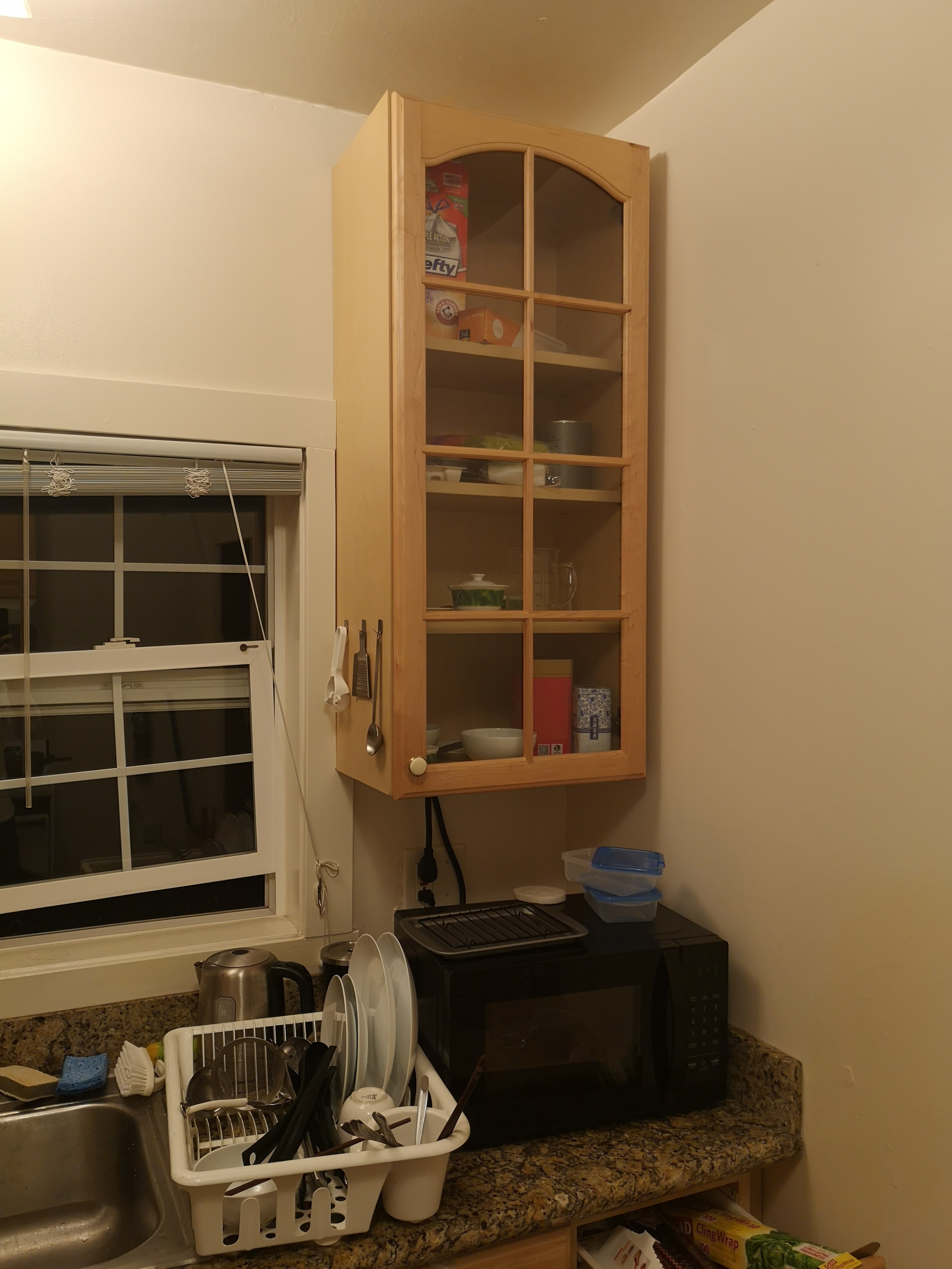
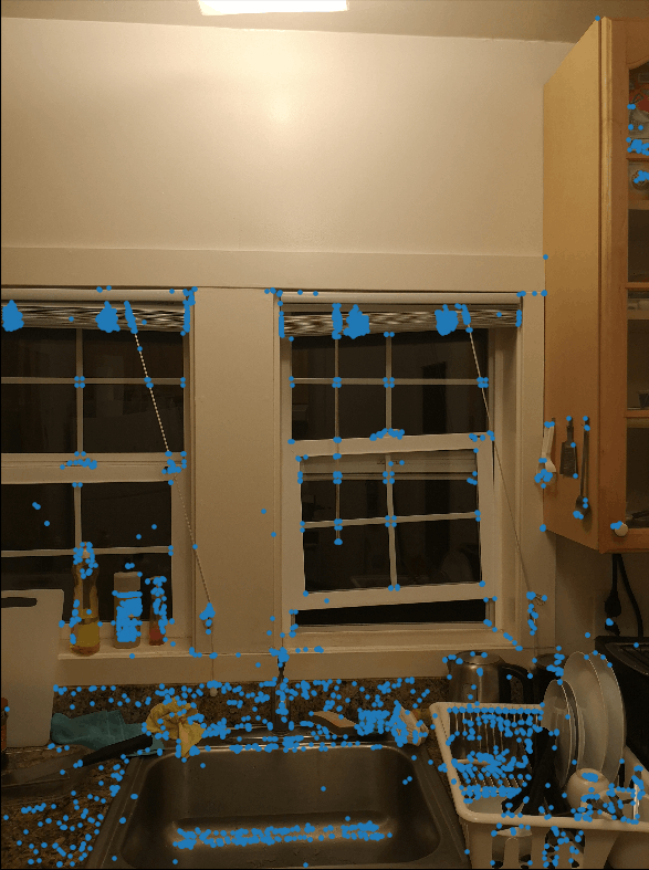
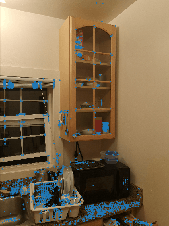
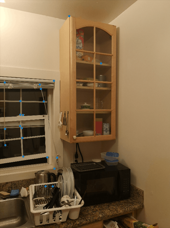
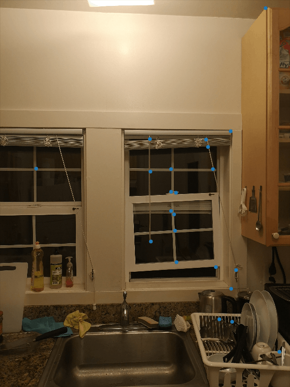
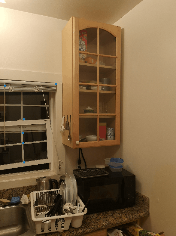
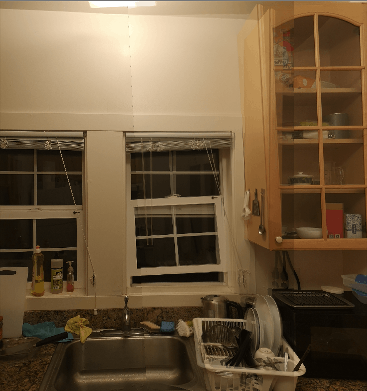
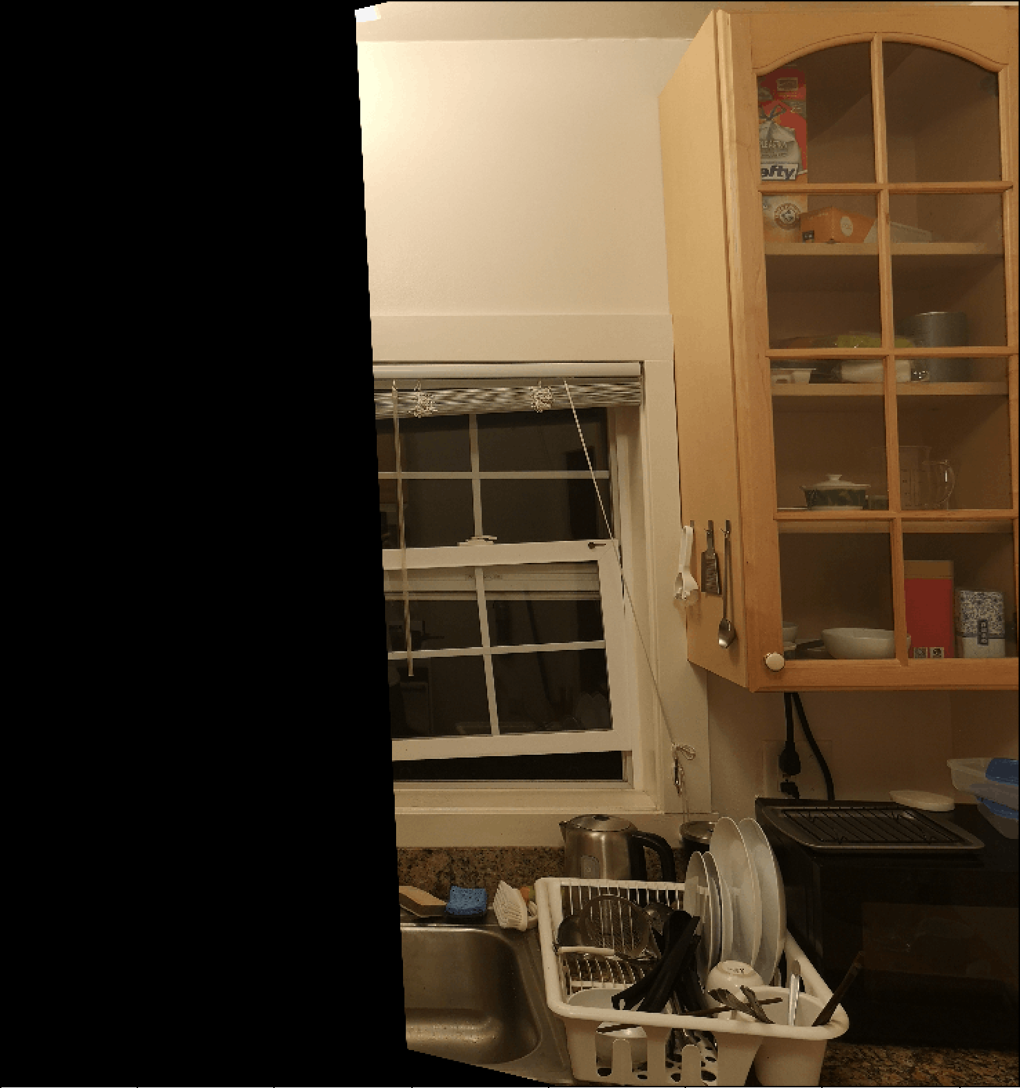
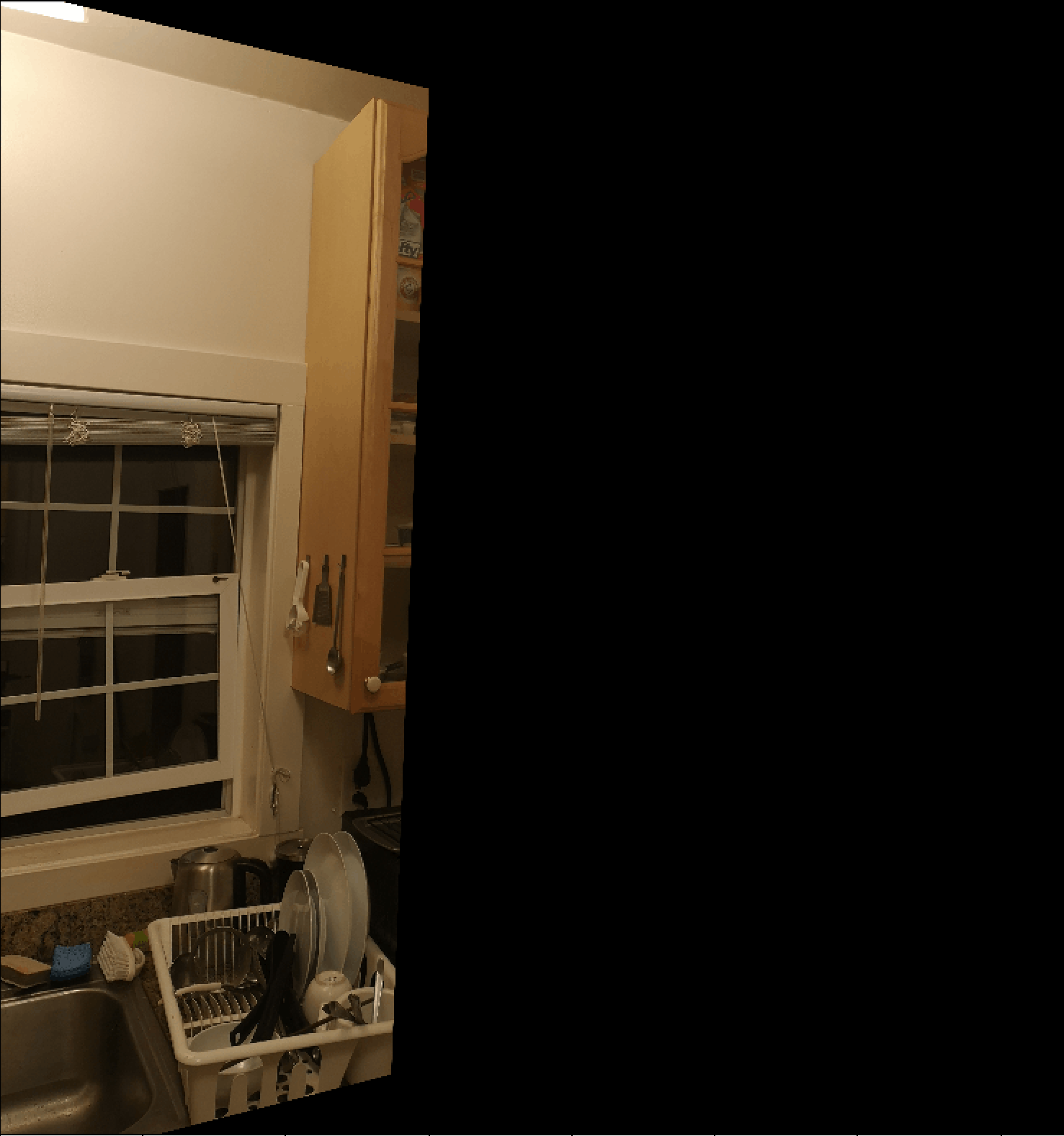
Here are two pictures taken from my kitchen from two different points of view.

Part 2: Recover Homographies

The idea of Homography comes from this website: http://www.corrmap.com/features/homography_transformation.php. We choose multiple pairs of corresponding points in both pictures, then use the formula in the website to get a least square solution of the transformation matrix.

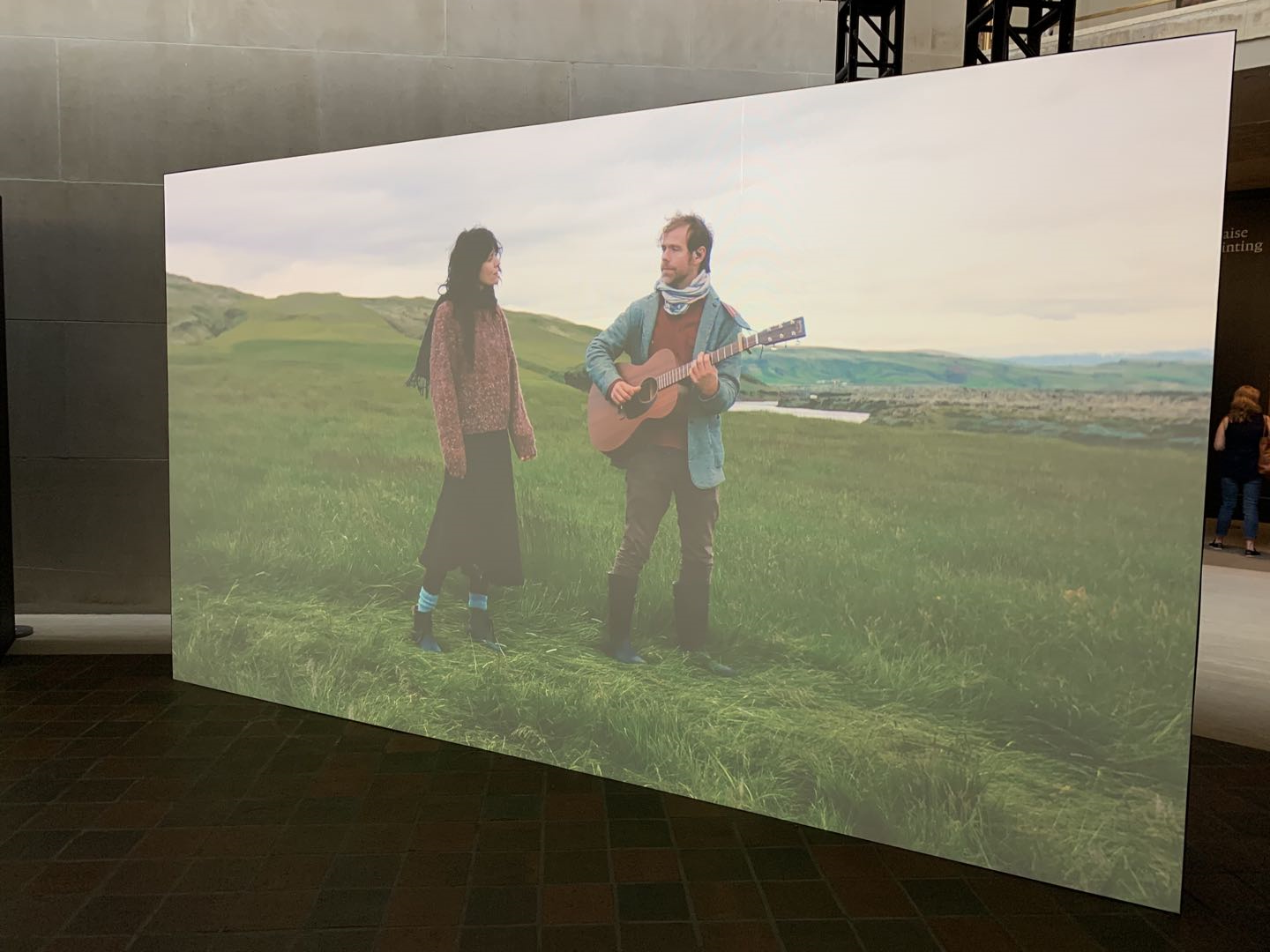
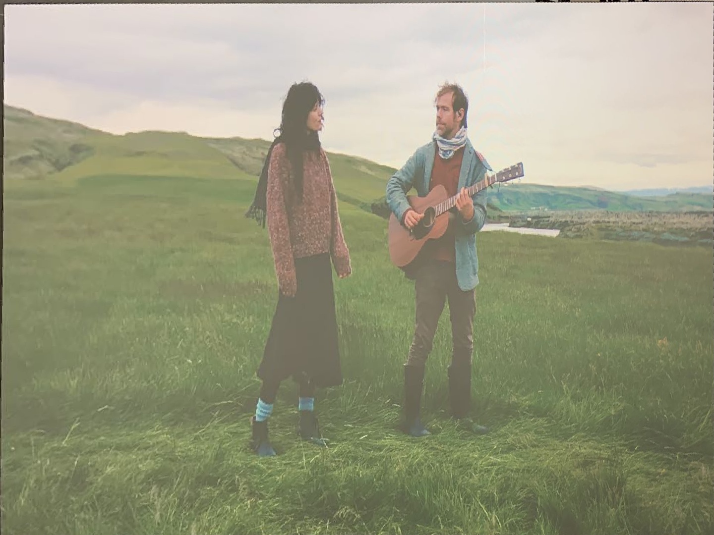
Part 4: Image Rectification

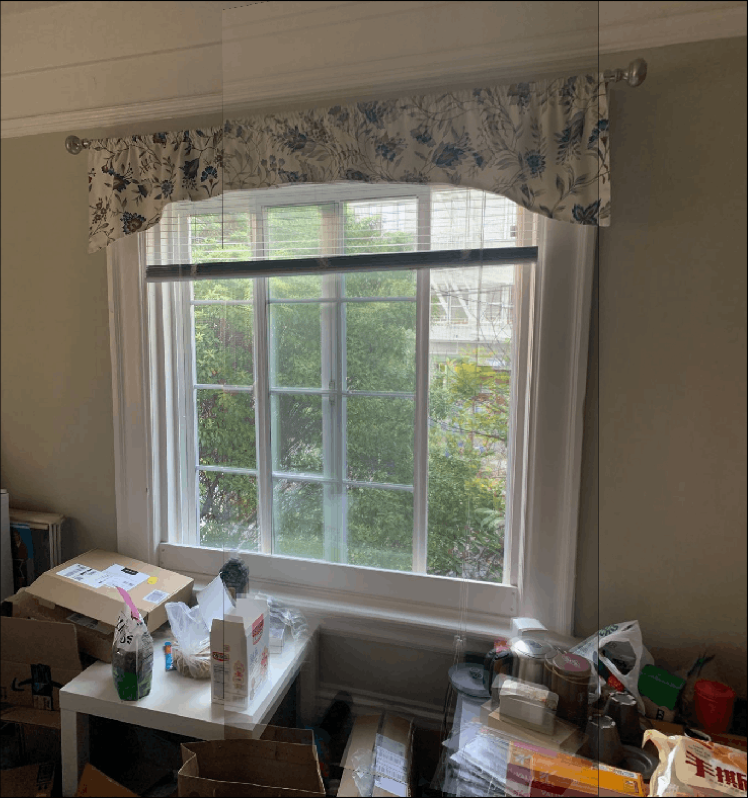
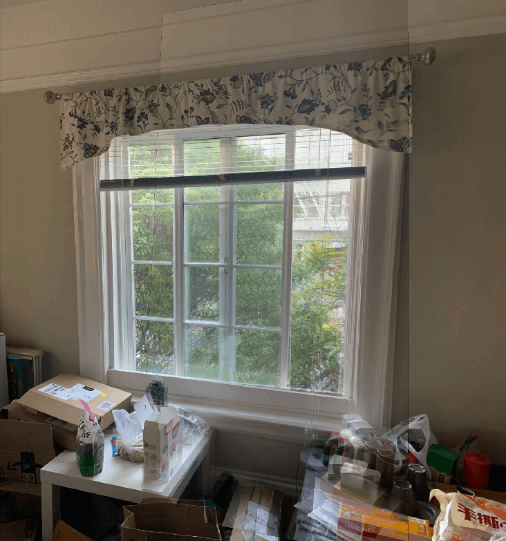
With the homogrtaphy, I pair the points on the four corners in a rectrangular screen in picture and pair them to the four corners of the picture.

Part 3: Warped the Images

Below is the cropped version of the left image toward the right image, and right image toward the left image.

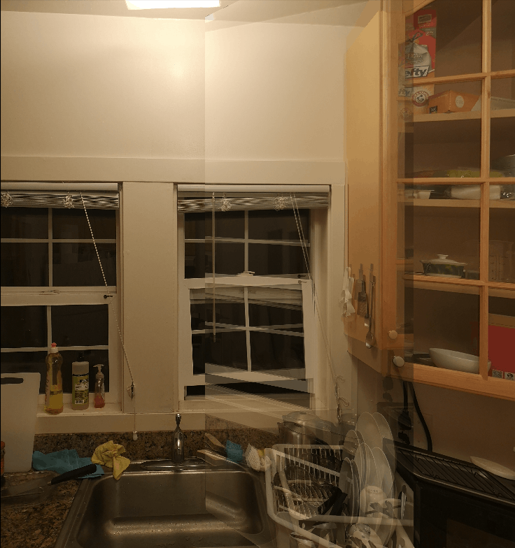
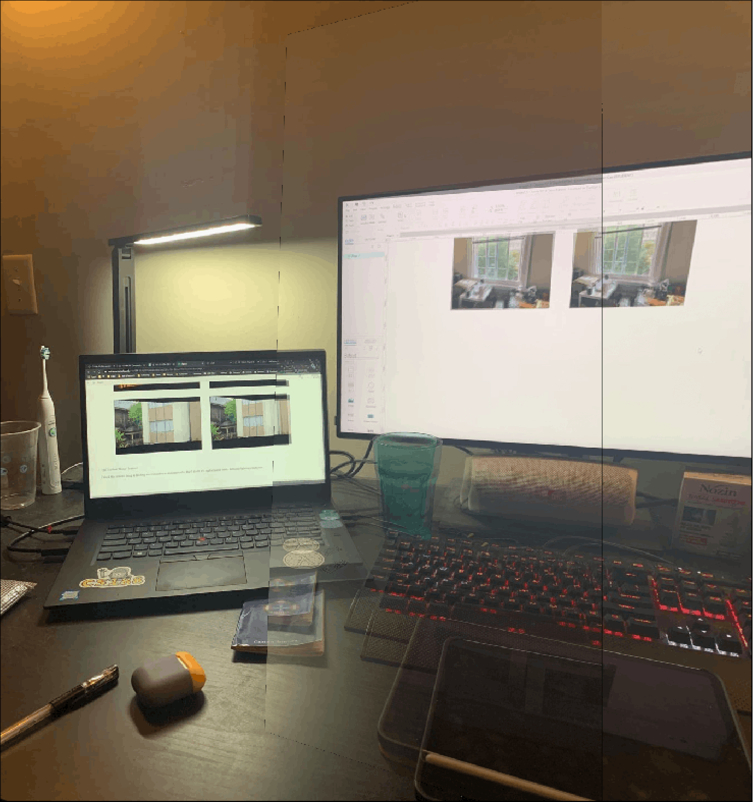
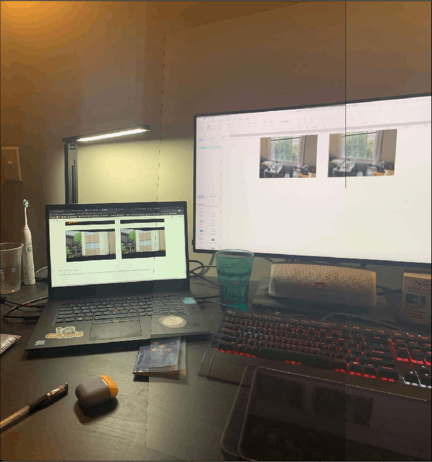
Part 5: Blending the Images into a Mosaic

Here is the result of blending the images. It is worth to notice that the warped image is darker than the original image. It is mainly due to the reason that in the process of transformation, some of the pixels are not mapped hence are filled with black. I will try to improve it in PartB.

Conclusion A:

Image Rectification is fun especially when you have the experience in the crowd museum that you don't have the chance to shoot the painting in a nice way. Image Rectification helps to solve this problem!

The following steps for auto stitching comes from the paper “Multi-Image Matching using Multi-Scale Oriented Patches” by Brown et al."

Step 1: Finding Harris Corners

We use harris interest point detectorto automatically detect corners in the image. I plot the top 2000 detected corners for each image.

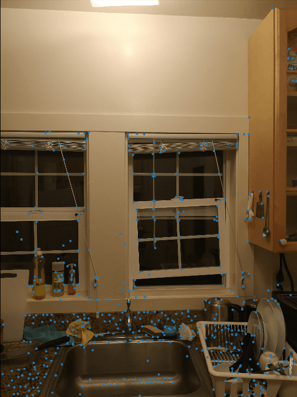
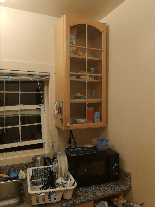
Step 2: Adaptive Non-Maximal Suppression

We select the 500 most promising corners using Adaptive Non-Maximal Suppression. We compute a suppression radius for each corner and select the top 500 corners with the highest suppression radius. The suppression radius of a corner is computed by its minimum distance to any other corner that has a higher corner strength. In this way, we make sure that the selected corners are most likely representing distinct and well-distributed features in the image. As in the paper, we choose c to be 0.9.

Step 3: Generate Feature Descriptors & Feature Matching

After finding the 500 interest points, we describe each of them using a 8*8 vector descriptor. We take the 40*40 neighborhood patch of each interest point and subsample it using the mean of each 5*5 block. Then, we normalize the 8*8 vector. After, we match points between the two images by computing L2 distance between pairs of features. For each feature, we compute the ratio of best and second best and reject with a threshold of 0.3.

Step 4: RANSAC

We run RANSAC to further distinguish correct matchings and incorrect matchings. We randomly choose four pairs of matchings, and compute a homography based on them. Then, we count how many inliers we would have given this homography transformation. After doing so for 10000 iterations, we keep the largest set of inliers we have found and compute a least-squares homography based on these inliers. We consider it to be an inlier if the distance between projected points and ground-truth points is less than 0.5.

Step 5: Auto Stitching

Continue what we did in part A. Below, left is the manual result, right is the automatical result. Both have fair results.

Conclusion B:

The coolest thing is that harris points, AMNS, feature selection and RANSAC free us from choosing correspondence. Both have similarly fair results.