Stitching Photo Mosaics
Overview
In this project, we use homographies to rectify and stitch images together.
Part 1: Rectification
In this part, we take an image of a planar surface at an angle and then use a homography ot straighten it out.


Part 2: Mosaics
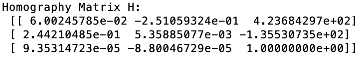
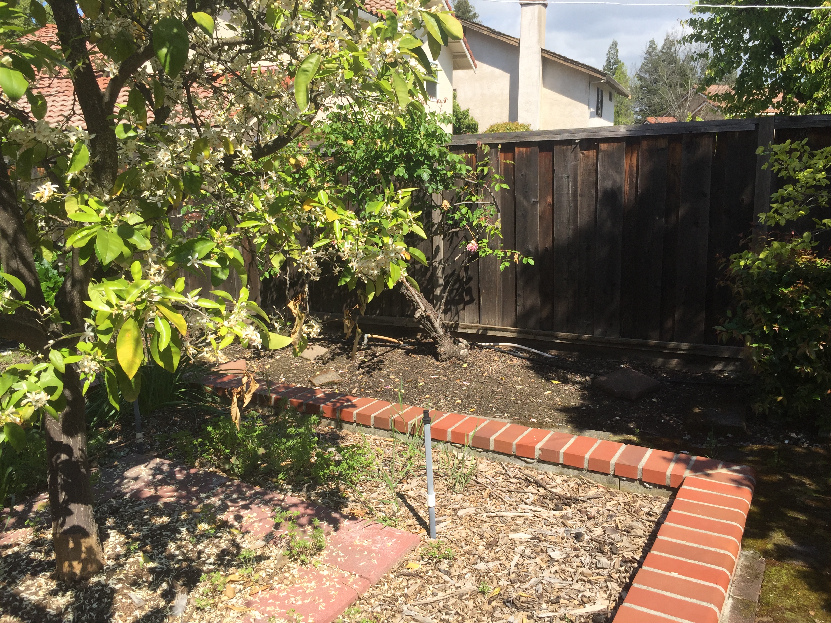
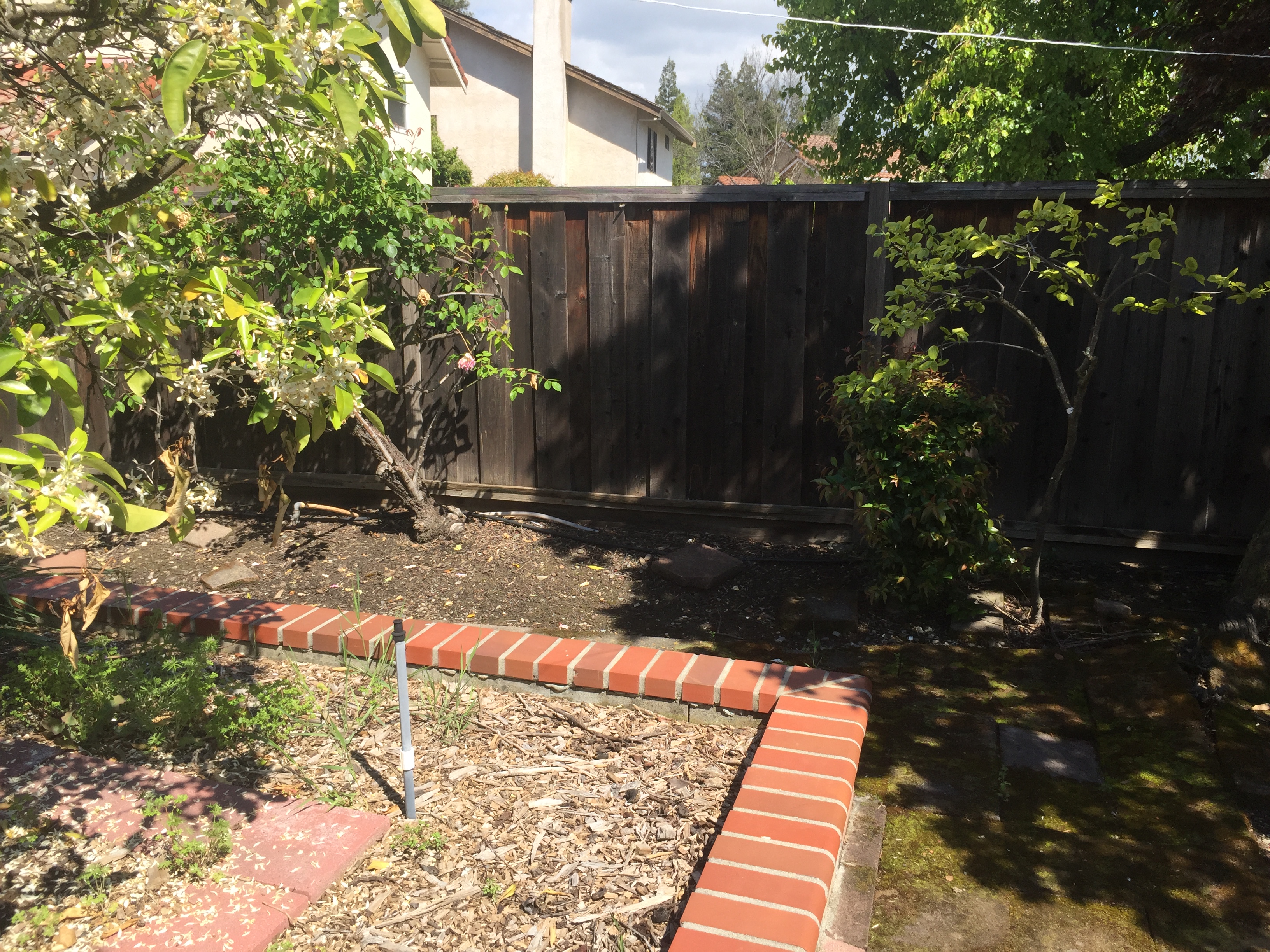
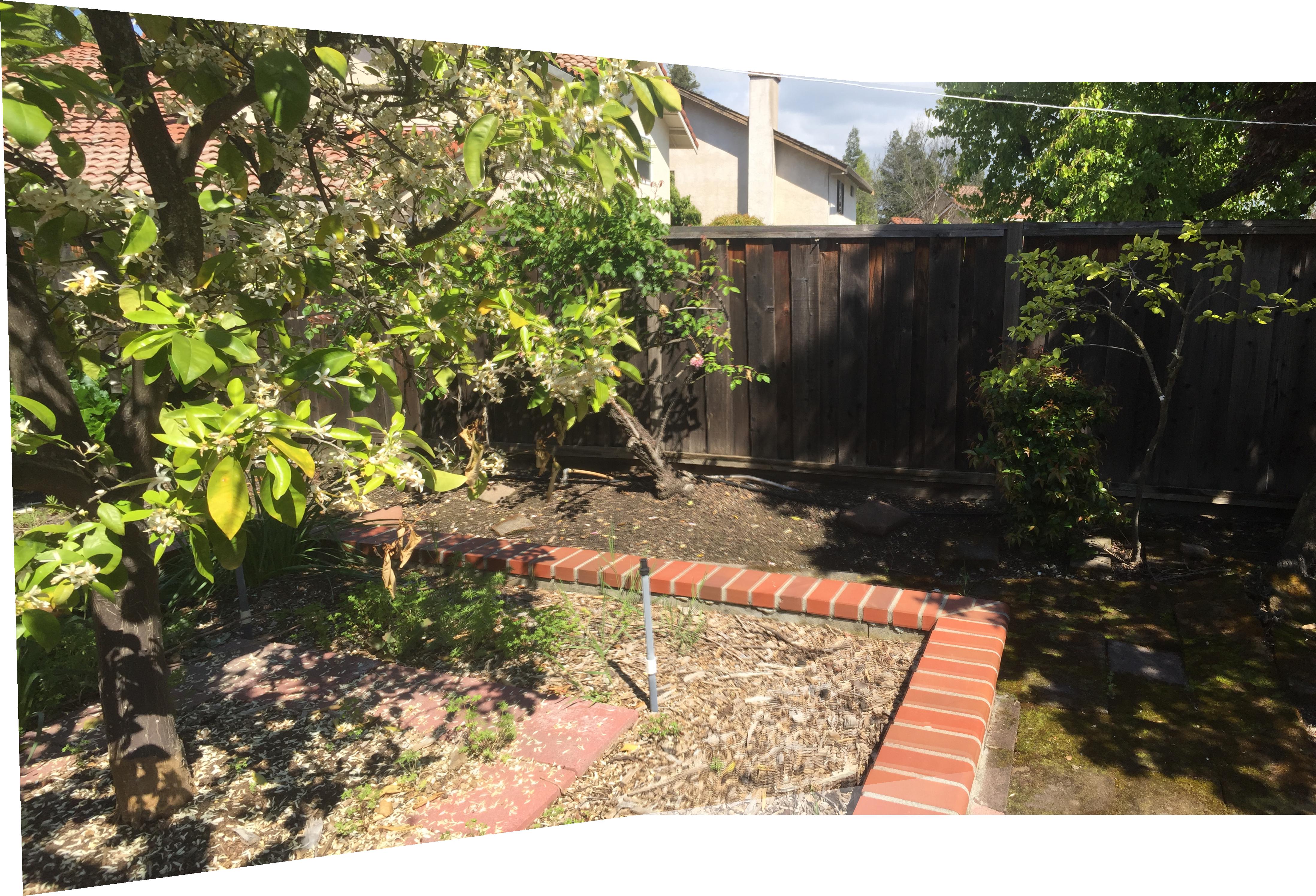
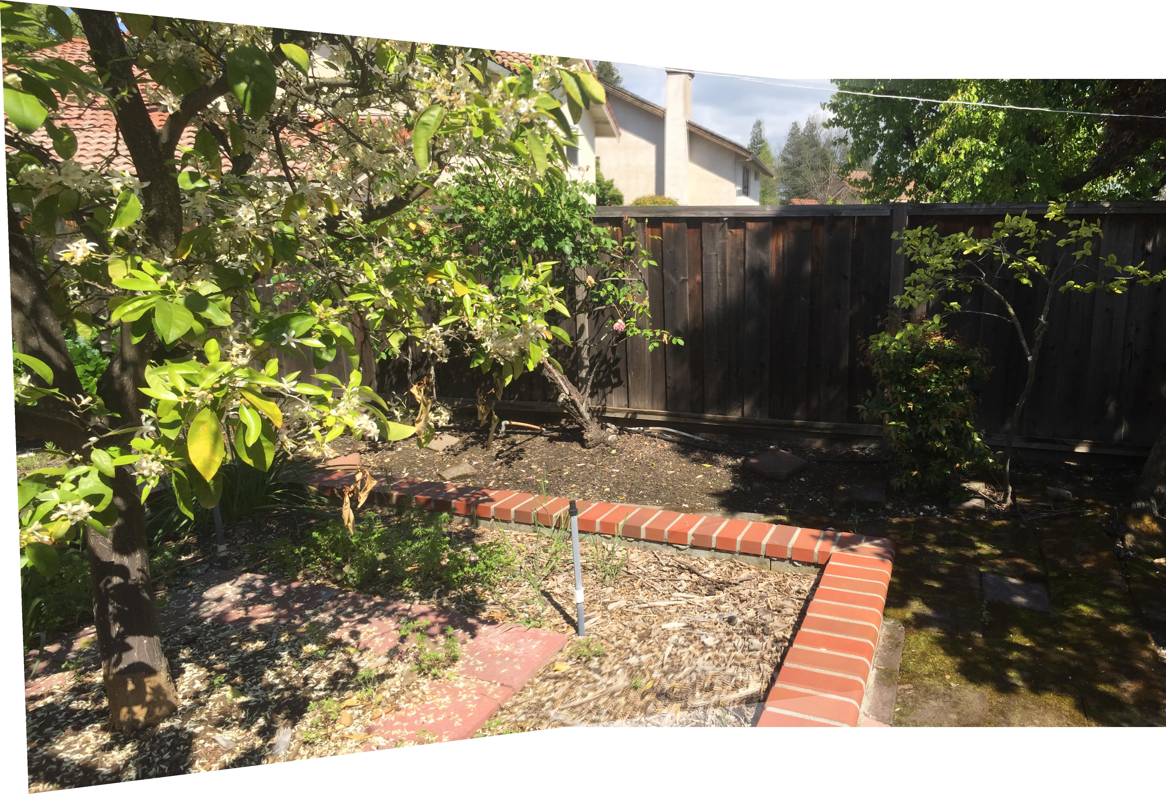
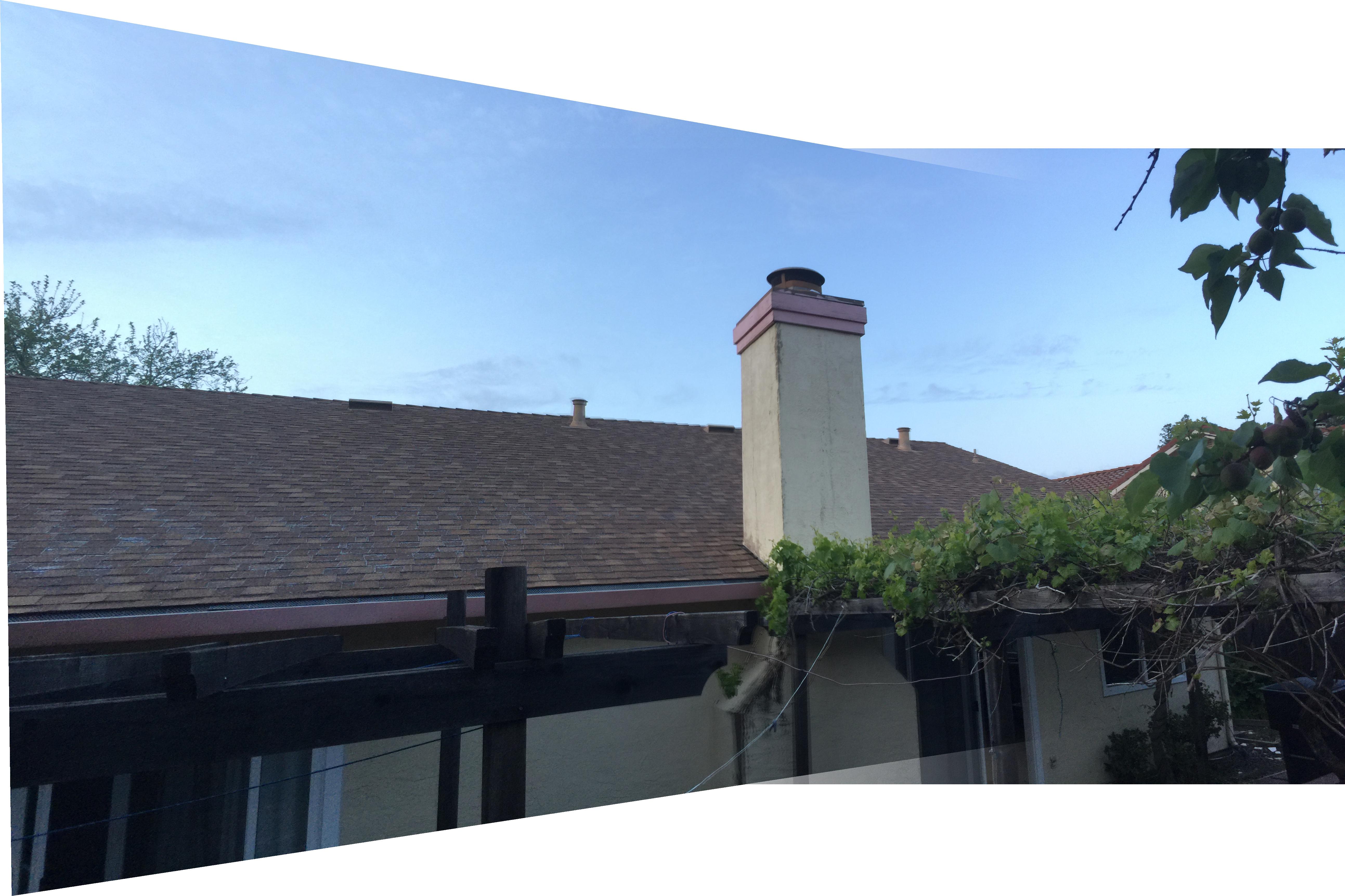
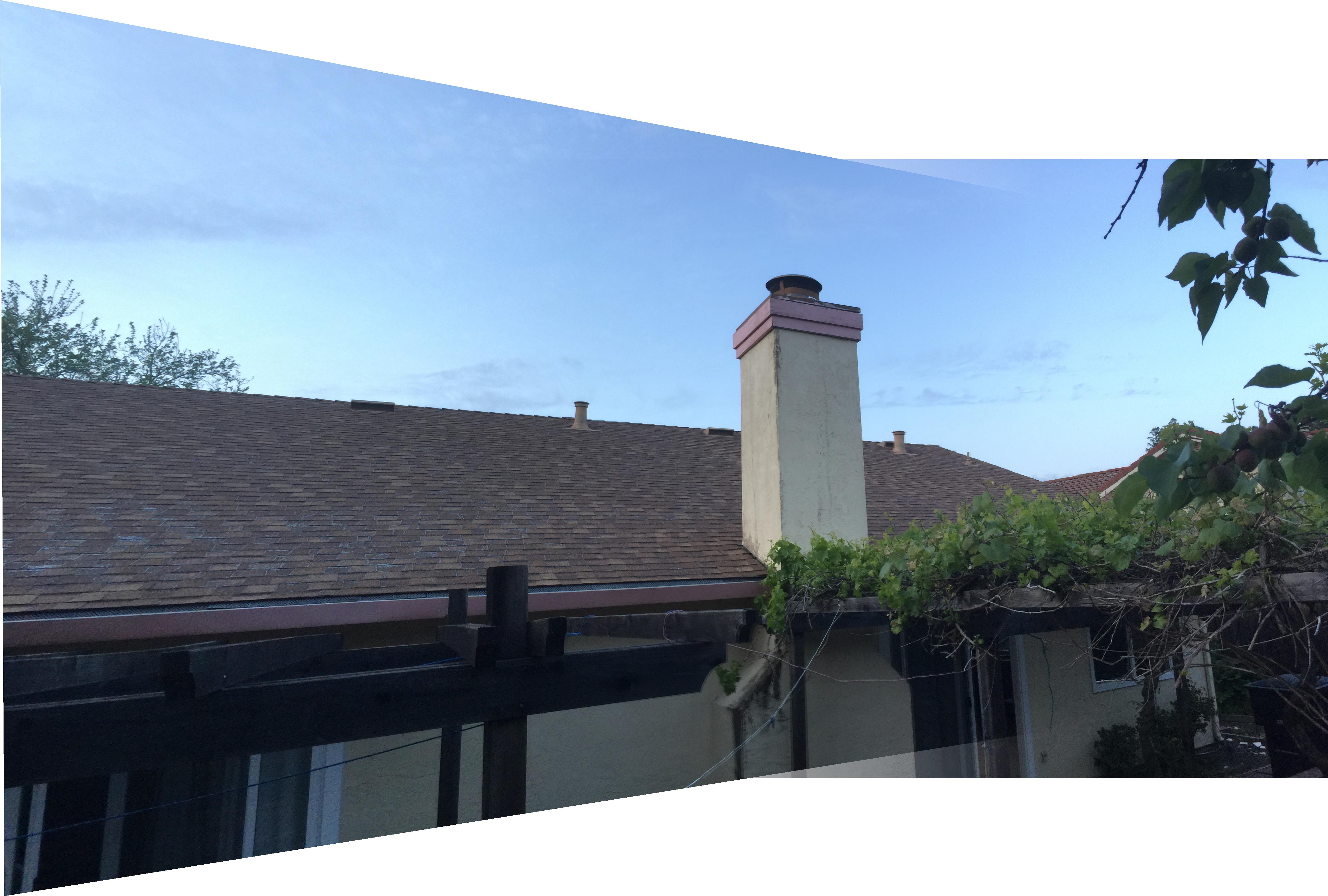
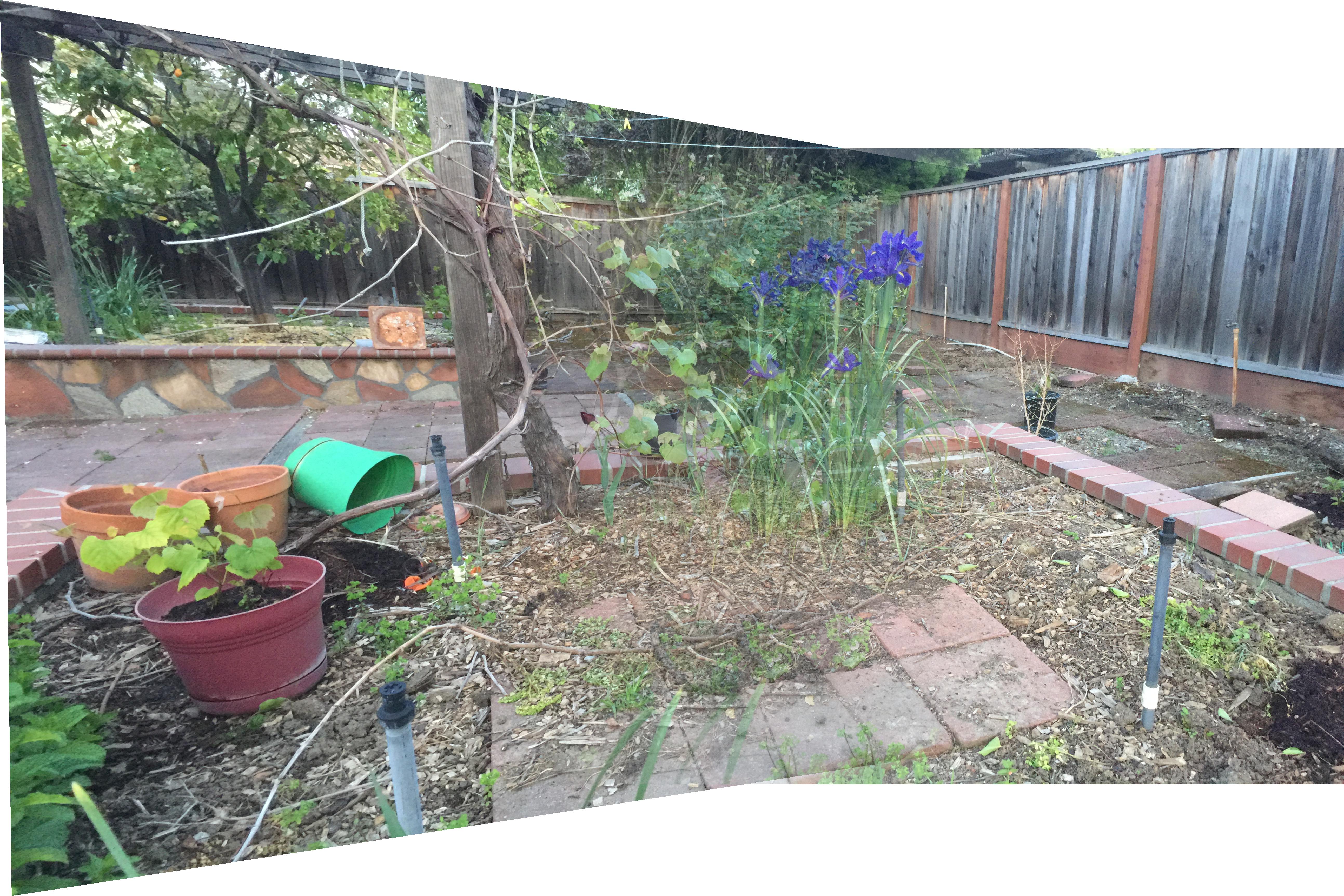
Here, we take two images from a single focal point (at different angles) and stitch them together. We use linear feathering where the images overlap to avoid vertical artifacting. I took some pictures from my garden.
Part B: Autostitching
Now, we adapt the program to select matching features automatically. The process is adapted from this paper: https://inst.eecs.berkeley.edu/~cs194-26/sp20/Papers/MOPS.pdf.
Feature Detection
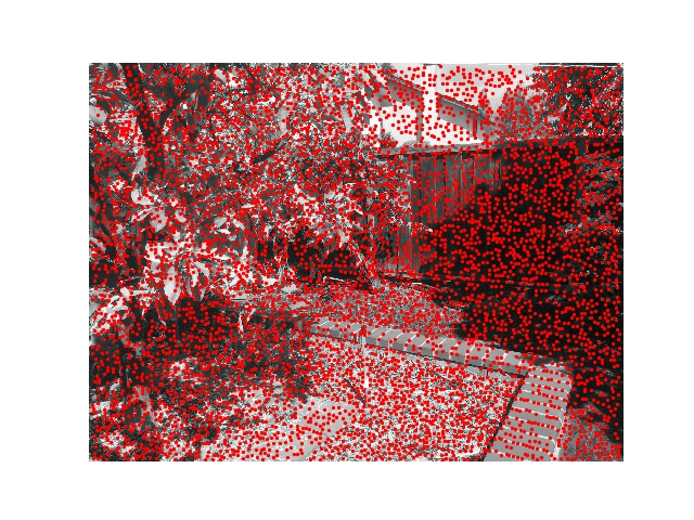
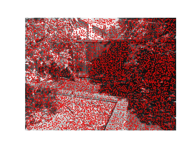
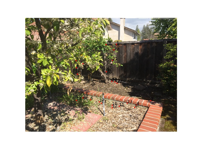
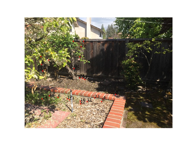
We begin by using the Harris Corner Detector to find all potential corners in our images. I increased the min_distance in peak_local_max to 15 to reduce the corner density. Here are all the potential corners in the garden images:
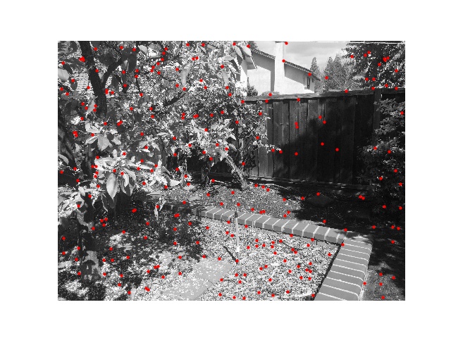
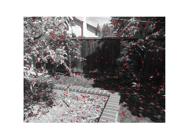
We then use Adaptive Non-Maximal Suppression (ANMS) to reduce the number of corners while maximizing their spread and intensity. We choose 250 coordinates with a c value of 0.9.
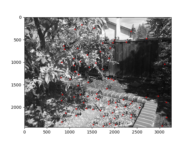
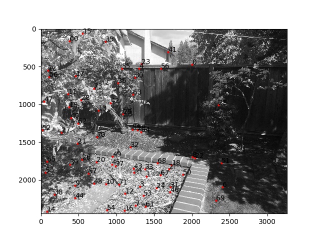
Feature Matching
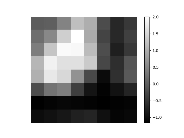
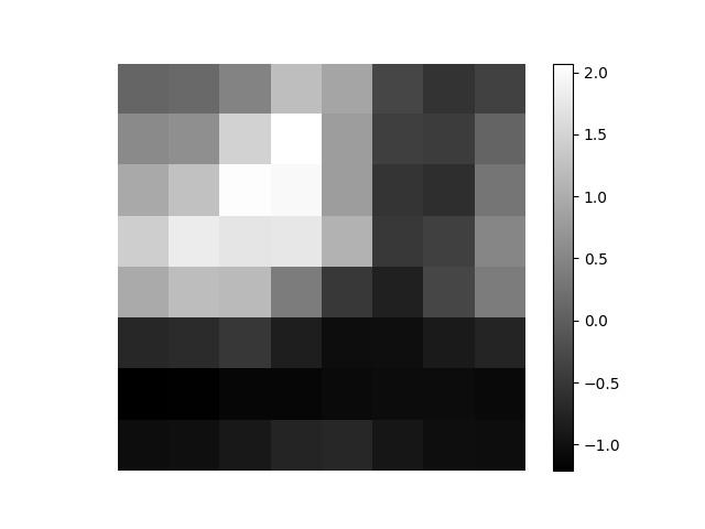
We then generate patches around each feature. We do so by first blurring the 40 x 40 square of pixels around each coordinate and then downsample the square to an 8 x 8 patch. Next, we calculate the SSD between all pairs of coordinates between both images. For each feature point in the left image, we calculate the ratio between its first nearest neighbor (1NN) and its second (2NN) in the right image. If the ratio is smaller than our threshold of 0.5 (meaning its much closer to 1NN than 2NN, indicating a likely match) we pair the coordinates. We throw away any unpaired coordinates. Below are sample matching feature patches and matching features.
RANSAC
We now have dozens of potential matching points between both images. The problem is that even a couple outliers can throw off our homography. We would prefer to keep just a handful of points that we know aren't outliers. We proceed with 10,000 iterations of Random Sample Consensus (RANSAC). In each iteration, we select 4 feature pixels randomly and calculate a homography. We then transform all matched features from the first image and check for inliers, which are pixels land up to 1 pixel away from their match in the second image. We keep the set with the most inliers. After RANSAC, we calculate our final homography using our maximal set of inliers. We can use this homography to transform images just like in part A.
Results
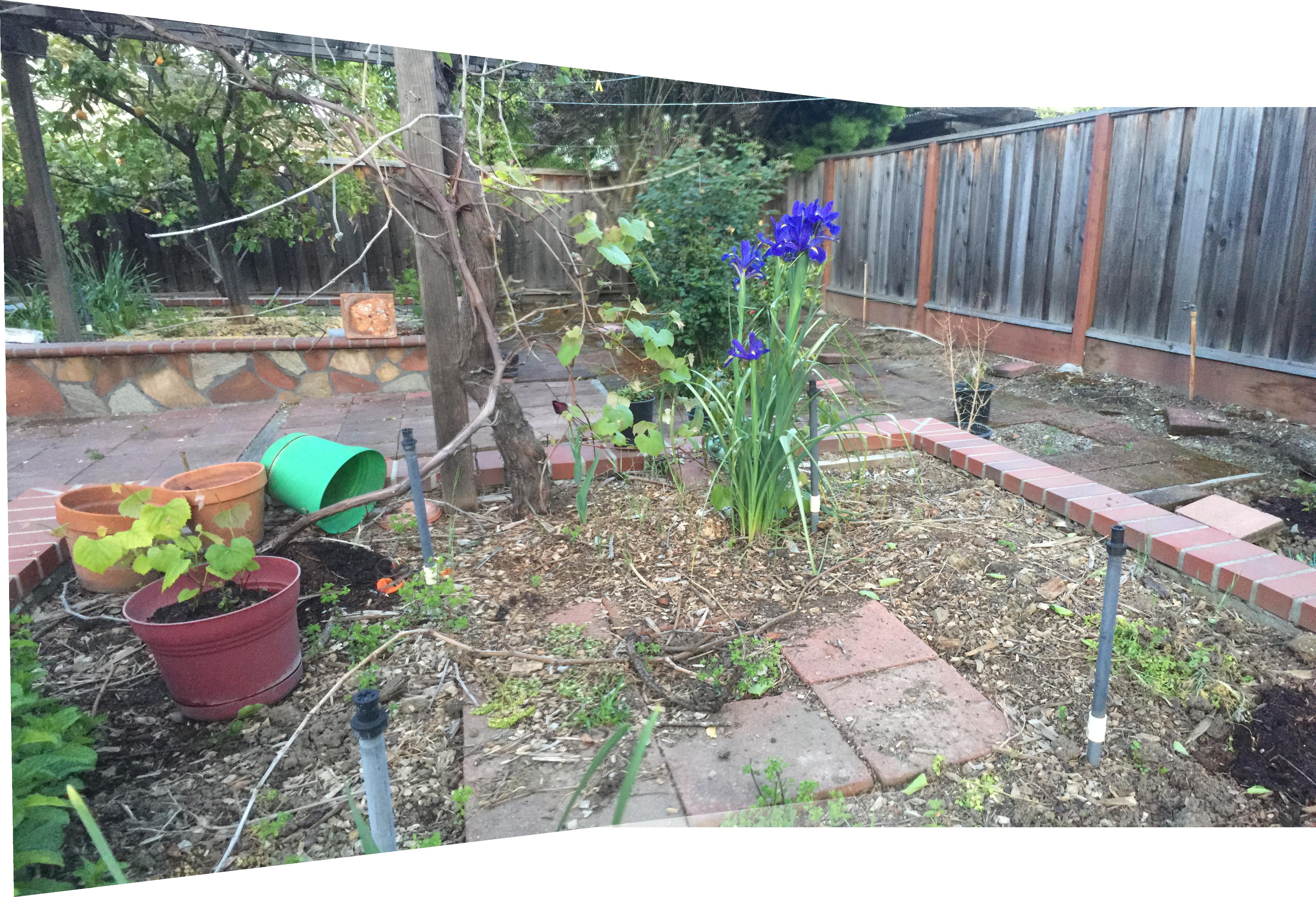
We compare our results between the manual and automatic panoramas. The auto aligned panoramas were better. In the flower for example, the manual alignment was far off, with a ghosting effect on the flower. On the other hand, the auto alignment effectively aligned the flower without such a stark ghosting effect.
Garden
Roof
Flower
Takeaways
I really liked this project. I thought the process of finding and filtering corners involved manipulating a lot of patterns in a really clever way. I especially liked learning about how we can use 8 x 8 patches to represent patterns independent of location in the image.