Part 1: Image Warping and Mosaicing
Overview
In this section, we utilize a homography transformation to rectify images and produce warped versions for image stitching. Here points are manually selected, but we will begin to uncover the secrets of auto-stitching in the next section.
How Do We Recover Homographs?
It's easy - you just call the function we defined for this section in main.py. What lies underneath the delicate numpy calls are significant amount of math.
Notice firstly that any two images on the same surface in space are related by a homography. Specifically, we define a \(3 \times 3\) homography transformation as follows:
This homography transformation has \(8\) degrees of freedom (as the last entry is fixed to be 1) and requires four correspondence pairs. Using only four correspondence pairs can be noisy, so we use more pairs. However, then, the system is overdetermined, and we use least squares to minimize:
$$\sum_{i=1}^{n} \lVert H \begin{bmatrix} x_{1,i} \\ y_{1,i} \\ 1 \end{bmatrix} - \begin{bmatrix} wx_{2,i} \\ wy_{2,i} \\ w \end{bmatrix} \rVert_2^2$$
Further algebra gives us that the matrix we solve for, then, is:
$$
\begin{bmatrix}
x_{2,1} \\ y_{2,1} \\ \vdots \\ x_{2,n} \\ y_{2,n}
\end{bmatrix}
=
\begin{bmatrix}
x_{1,1} & y_{1,1} & 1 & 0 & 0 & 0 & -x_{1,1} x_{2,1} & -y_{1,1} x_{2,1} \\
0 & 0 & 0 & x_{1,1} & y_{1,1} & 1 & -x_{1,1} y_{2,1} & -y_{1,1} y_{2,1} \\
& & & & \vdots & & & \\
x_{1,n} & y_{1,n} & 1 & 0 & 0 & 0 & -x_{1,n} x_{2,n} & -y_{1,n} x_{2,n} \\
0 & 0 & 0 & x_{1,n} & y_{1,n} & 1 & -x_{1,n} y_{2,n} & -y_{1,n} y_{2,n} \\
\end{bmatrix}
\begin{bmatrix}
a \\ b \\ c \\ d \\ e \\ f \\ g \\ h
\end{bmatrix}
$$
Image Rectification
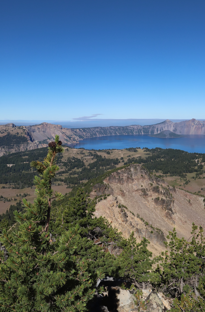
We take images and rectify them. This is done by computing the homography matrix from original image (manually selected points) and a rectangle.
 Original Photo (link)
|
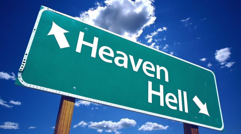
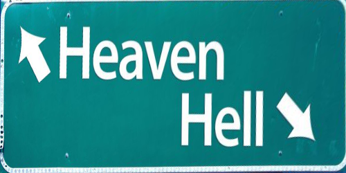 Rectified Photo (Interesting Sign!)
|
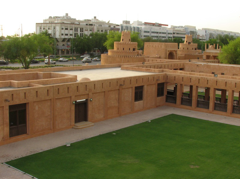
 Original Photo
|
 Rectified Photo (I promise I was paying attention)
|
Mosaics
Given images with the same point of view, but rotated viewing angles and overlapping fields of view, we can create a mosaic of the images to create a panorama. To do this, we will recover the homography as above, and warp the images to the center image, then blend the resulting warps.
Part 2: Automatic Stitching
Overview
In this section, we take our work from Part 1 and extend it to automatically stitch together multiple images.
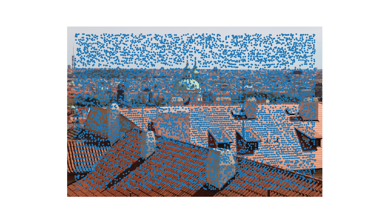
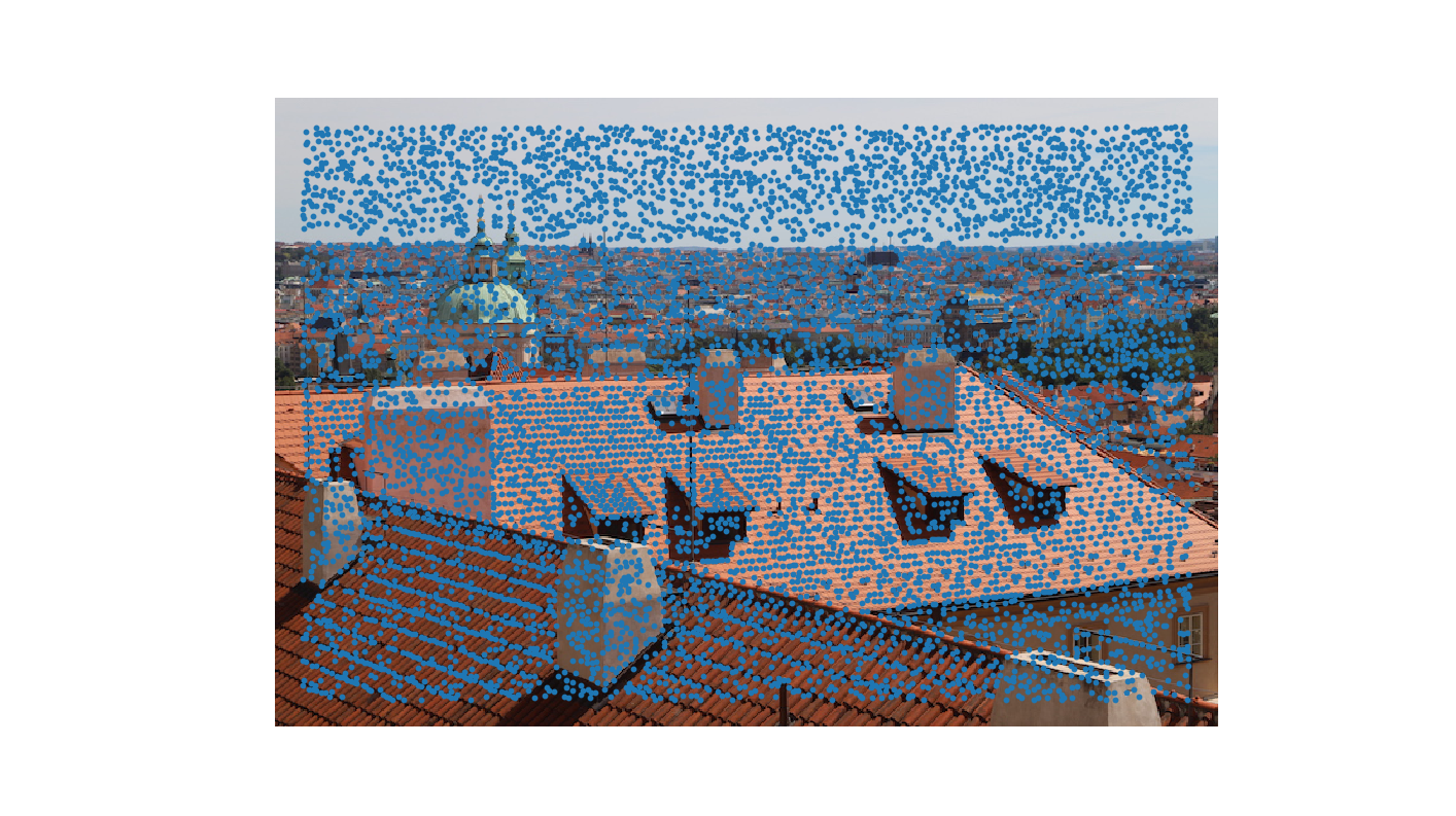
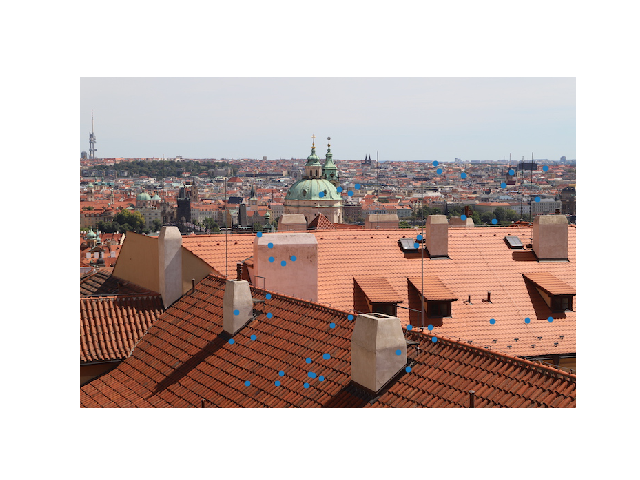
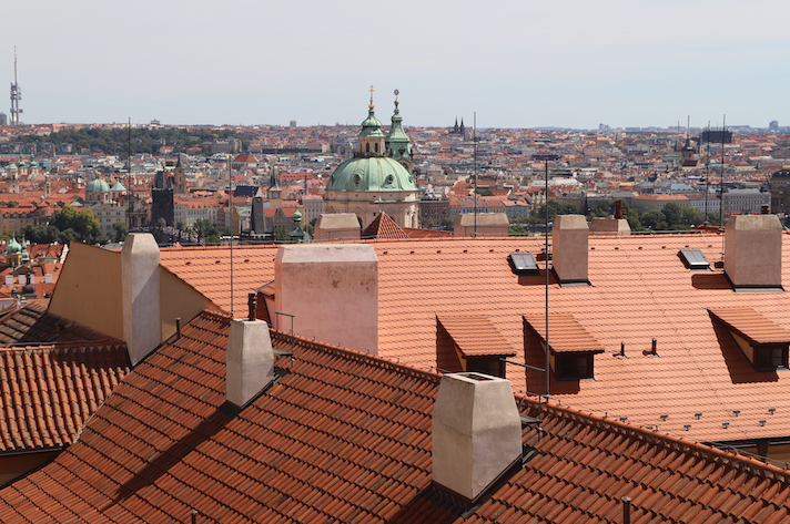
Harris Corners
To find matches between images, we need to generate potential points of interest. To do so, we use Harris Corner Detection to find corners in an image, where corners are defined by points whose local neighborhoods stand in two different edge directions. Below, we show two images with their Harris Corners overlaid:
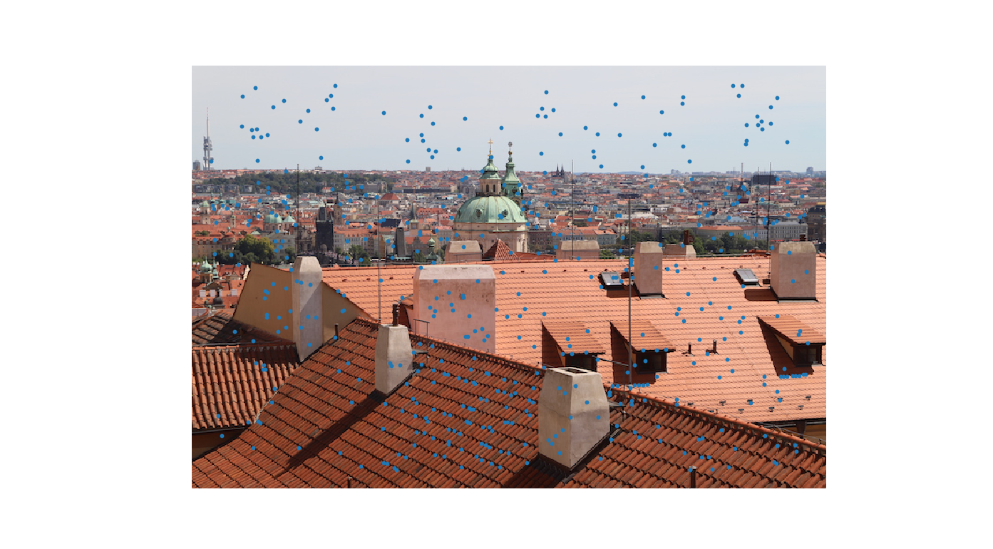
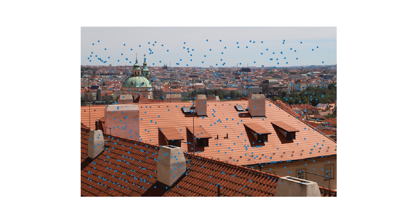
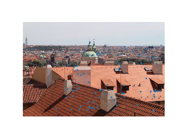
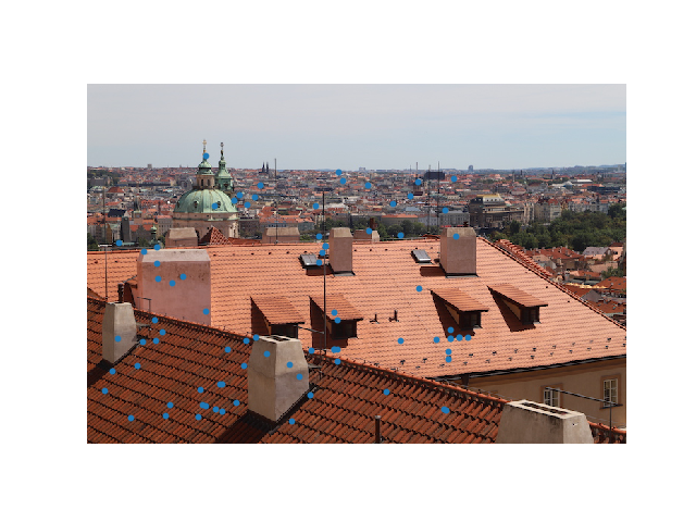
Adaptive Non-Maximal Suppression (ANMS)
Using Harris Corner Detection algorithm returns too many points of interest. To remedy this issue, we turn to ANMS to limit the maximum number of interest points extracted from each image. At the same time, we notice that these points are not necessarily distributed spatially. ANMS solves these issues by sorting points by non-maximal suppression radius. In my implementation, I use \(c_{robust} = 0.9 \) and keep only the top \(500\) points (as sorted by non-maximal suppression radius). Below, we show the results after running ANMS:
Multi-Scale Oriented Patches: Feature Descriptor Extraction
We now use our interest points as feature descriptors, which should be invariant and distinctive. We use Multi-Scale Oriented Patches (MOPS). Specifically, we take \(40 \times 40 \) pixels and rotate it to a canonical orientation and subsample to \(8 \times 8\) to eliminate high frequency signals. Then, we normalize the subsample. This makes the features invariant to affine changes in intensity (bias and gain).
Feature-space Outlier Rejection: Feature Matching
we compute the squared distance from every feature in the first image to every feature in the second image. Then, we use the David Lowe's trick and compute the ratio of the distance to the 1-NN over the distance to the 2-NN. If this is less than \(0.3\), then the pair is a match.
Random Sample Consensus (RANSAC)
The RANSAC loop runs by firstly selecting four features at random (four since it is the minimum set of feature pairs for a homography). We take the minimum since we will have more chance of wrong pairs being chosen. We then compute the homography and count the inliers:
$$dist(p_i', Hp_i) < \epsilon$$
In our case, the distance metric was the \(L2\) norm. We repeat this while keeping the largest set of inliners (inliners defined to have SSD error lower than threshold \(0.8\)) and recompute least squares estimate on all of them.
Results of Automatic Stitching
We extend our studies further beyond the city picture to automatically stitch other photos. We provide the manually stitched photos for comparison on the left. To the right are the automatic stitched photos (they look almost identical! - more on this reflection soon). To make the pictures look better, they have been manually cropped to a rectangle.
What I learned
I am beyond surprised that automatic stitching and manual stitching returned almost identical results. The biggest thing I have learned is how to do feature extraction and feature matching, but more importantly, how simple ideas like using patches and normalizing can be used to create beautiful panoramas.