Part 1
For this project, we we were tasked to create image mosaics. To do this, we first need to compute the homography between the images, apply it so that they "line up", then merge them together. The tough part comes with computing the best possible homography. In Part 1, we show how, by manually choosing correspondences, we get pretty good results and can even do cool things such as image rectification, where we can view different parts of an image at different angles. In part 2, we make this process more robust, by automating the feature selection process, and we see that this leads to improved results.
To get the homography, we need a mininum of 4 point correspondences. However, these are very susceptible to noise, so instead, we can get a least-squares estimate instead.
1.1 Image Rectification
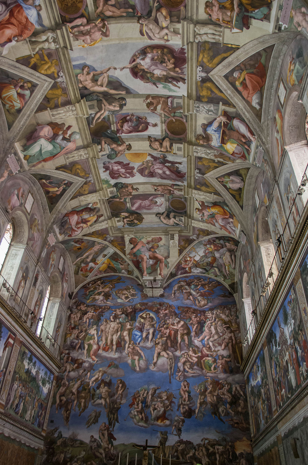
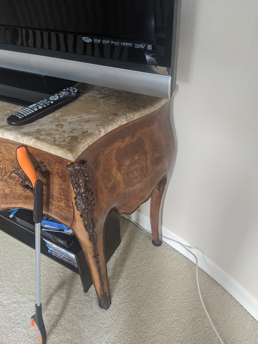
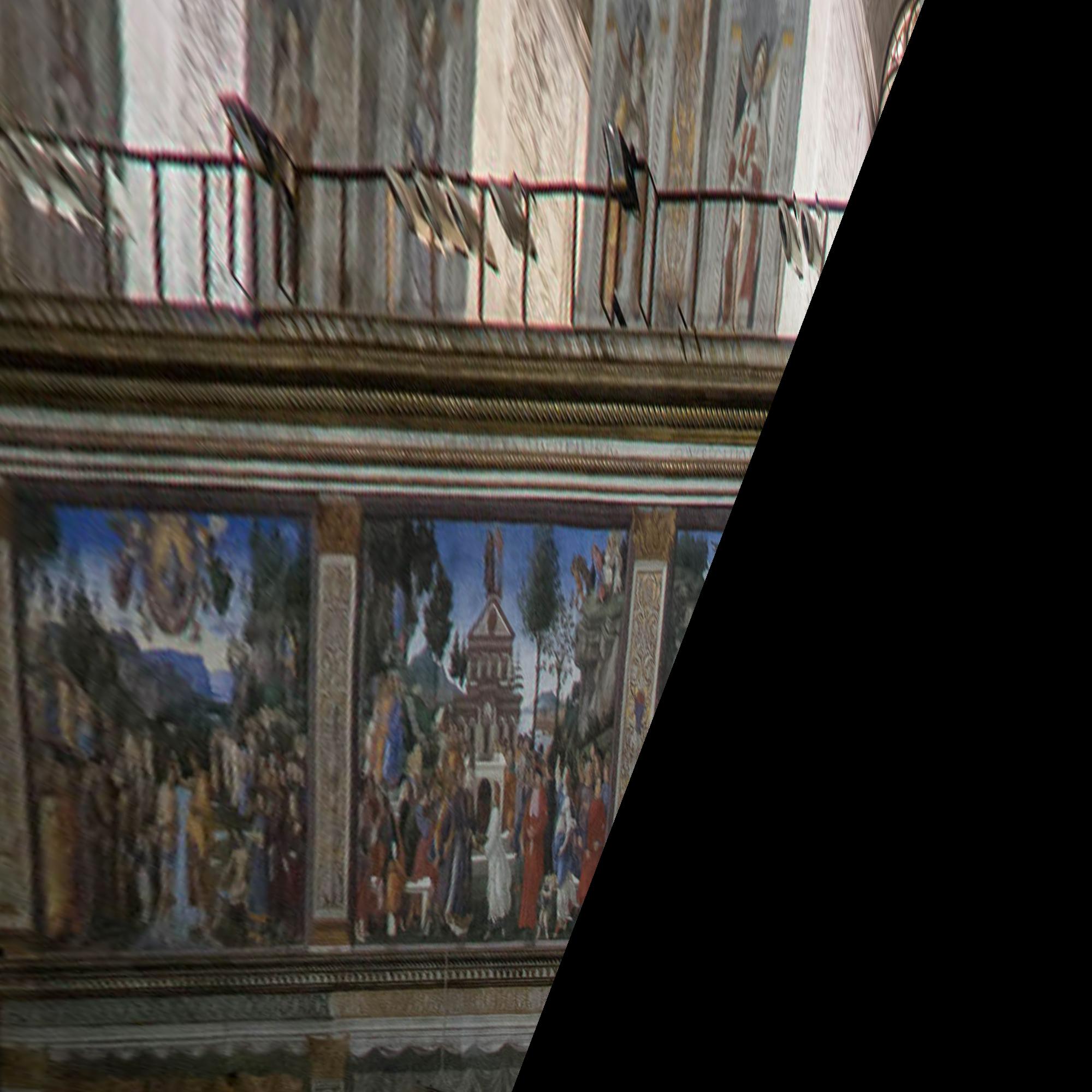
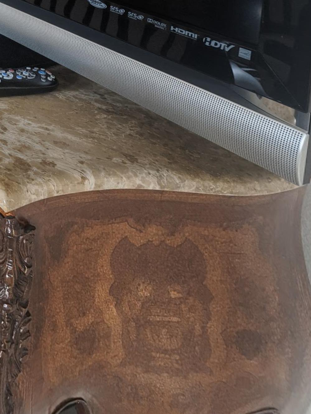
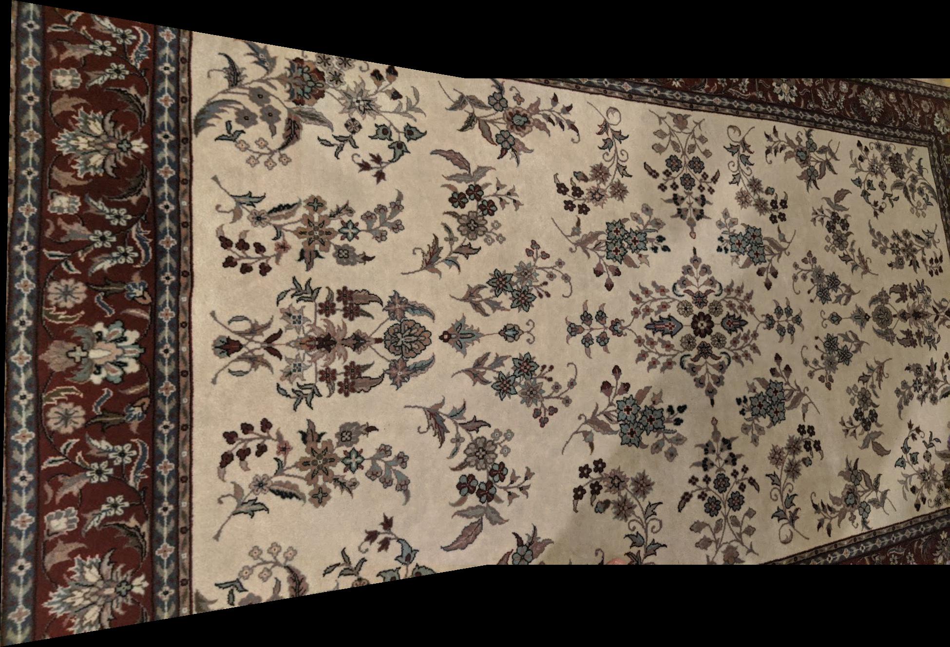
In order to rectify an image, we simply choose the 4 corners of the area we care about, and make those the corners of the "blank" output image we wish ot map to. Below, you can see the results of doing this on the Sistine Chapel and a table in my house. Wow, what a weird angle. I wanted to see what the paintings on the right wall were! Well, with the power of image rectification, we now can!
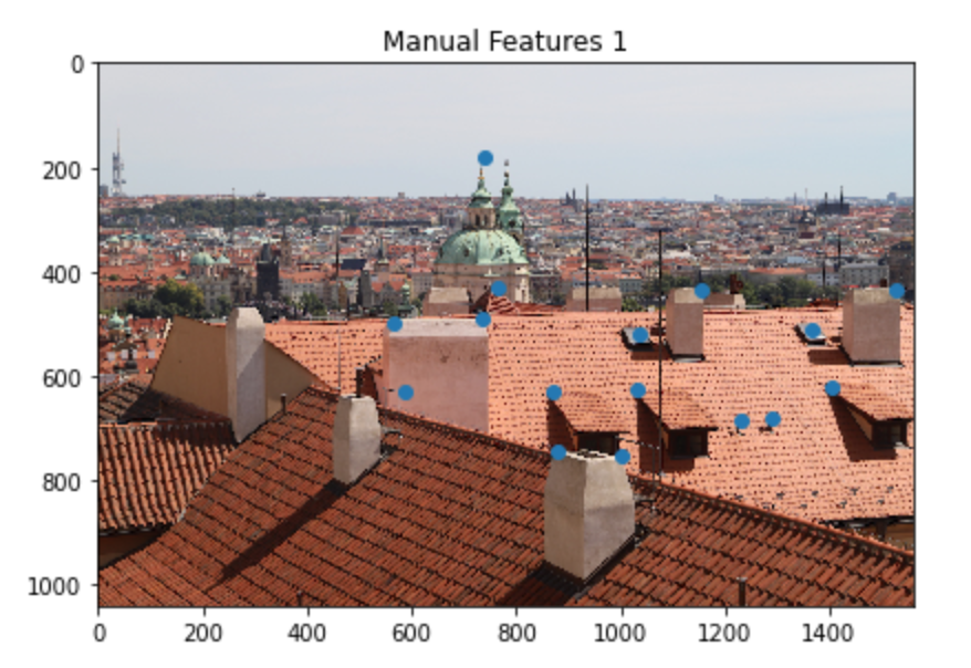
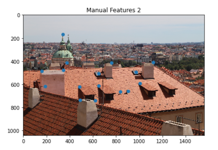
1.2 Manual Pano
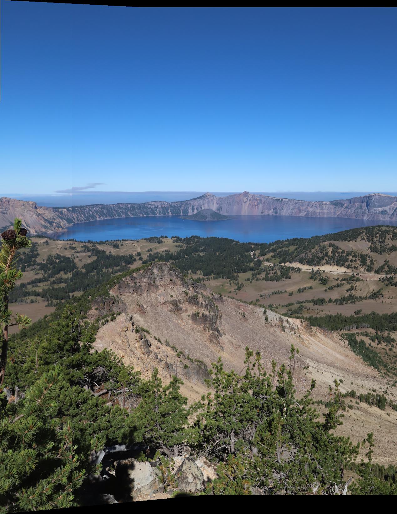
Here is an example of a panorama I made by manually using feature points. As we can see, it doesn't do the greatest job as the tiles on the roof in the bottom aren't lined up.
Part 2
For this part, to save ourselves from having to manually choose features each time, we decided to use the methods described in Multi-Image Matching using Multi-Scale Oriented Patches (Brown, Szeliski, Winder) to automate the process. Below you can find what each step looked like on an example.
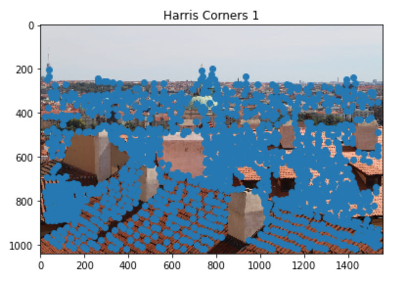
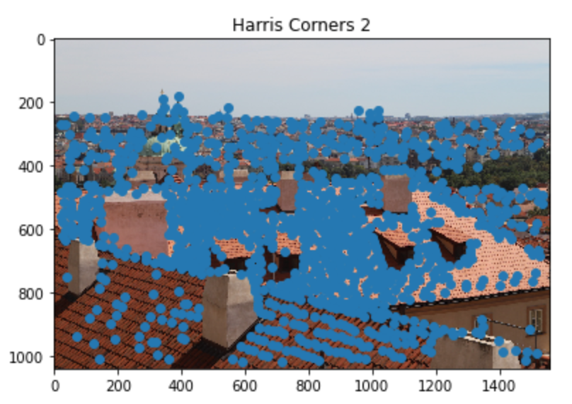
2.1 Harris Corners
The first step is to extract the Harris corners of each image.
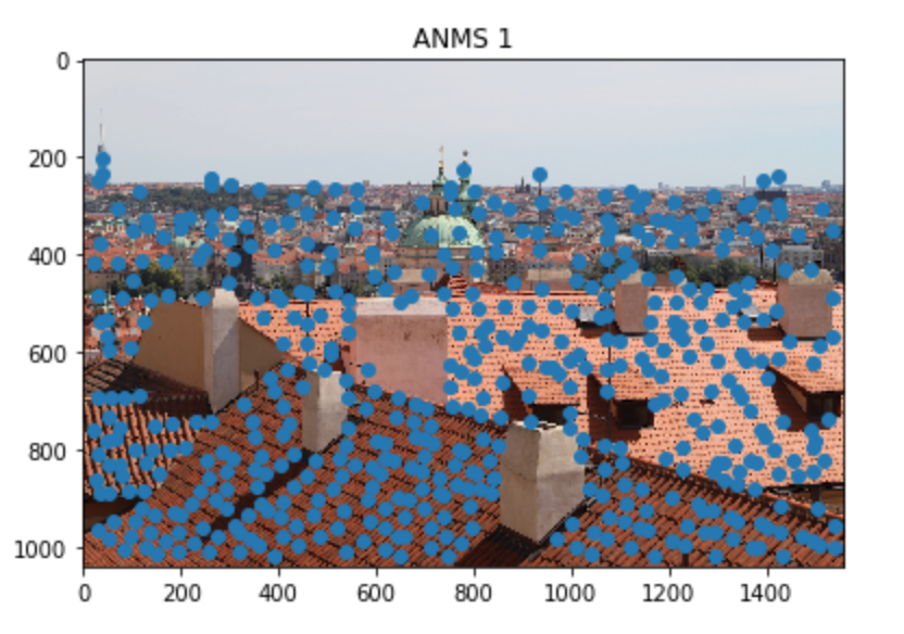
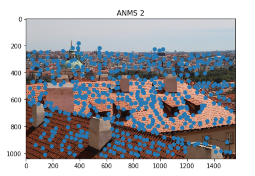
2.2 Adaptive Non-Maximal Suppression
Clearly we have too many points. To get rid of them and ensure that we have a good spatial distribution of points, we utilize ANMS, which finds points that are furthest away from the next closest point. I decided to keep the top 500 points.
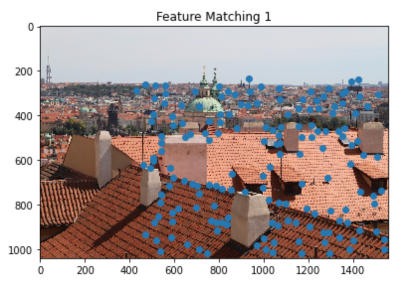
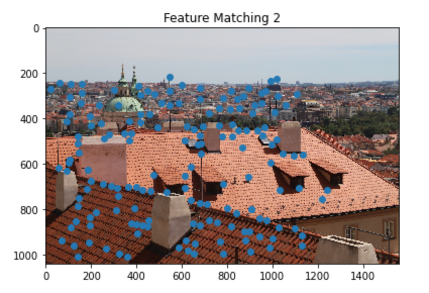
2.3, 2.4 Feature Descriptor Extraction and Matching
From here, we now need to get rid of points that exist in one image but not the other. We accomplish this using feature descriptors: take a 40x40 patch around each point, downsample to 8x8, then find the closest respective 8x8 patch in the second image. To differentiate what is "good", we utilized Lowe's technique of using the ratio of the First Nearest Neighbor error divided by the Second Nearest Neighbor error. I used a threshold of 0.5.
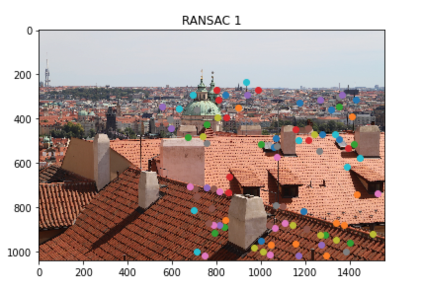
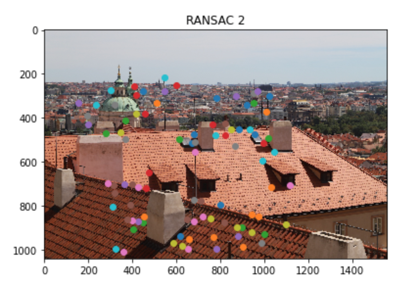
2.5 RANSAC
Finally, we can compute our homography estimate. However, there may still be outliers lurking around, so we use RANSAC to find the best estimate. I ran it for 10,000 interations with an epislon of 3.
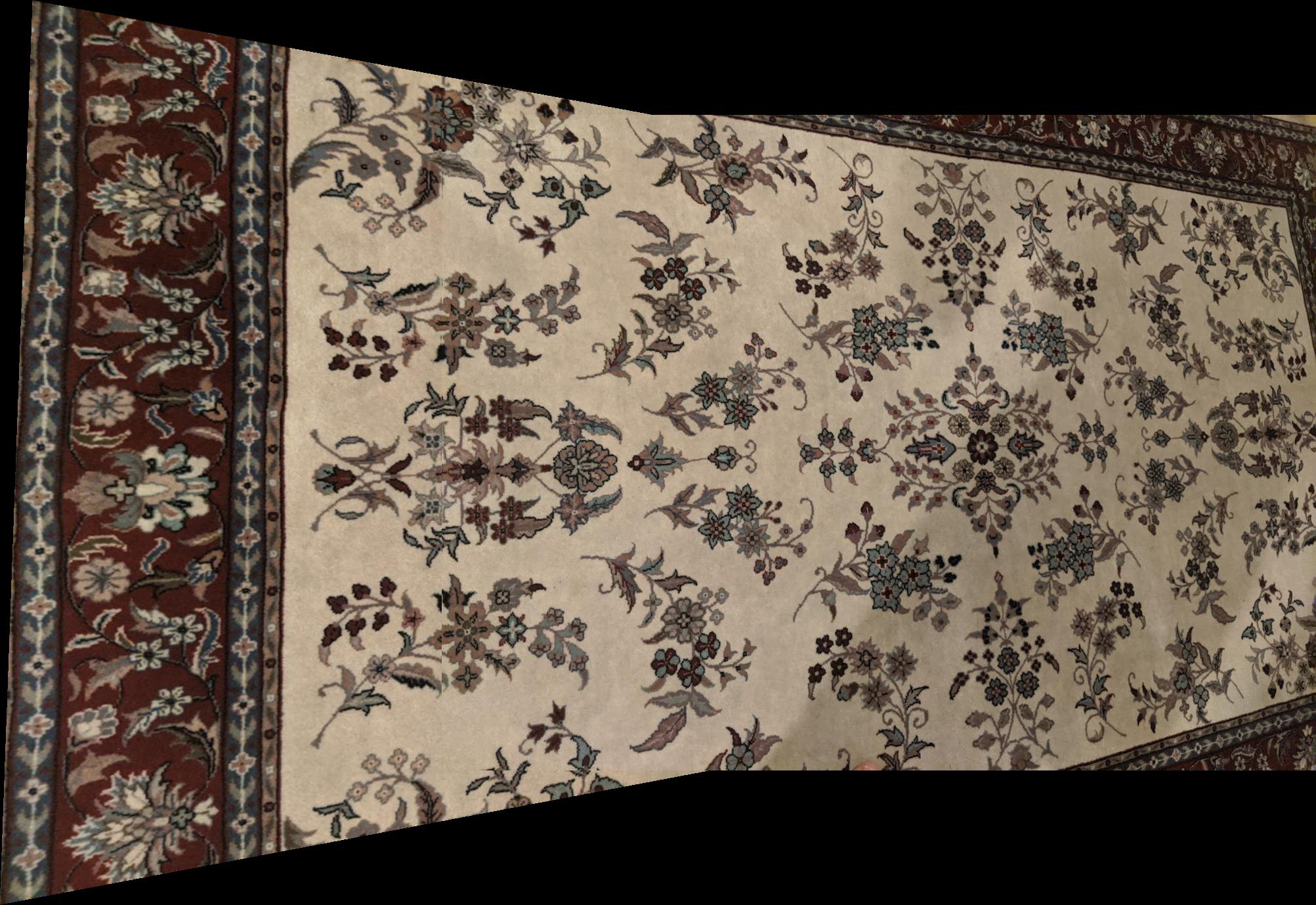
2.6 Results
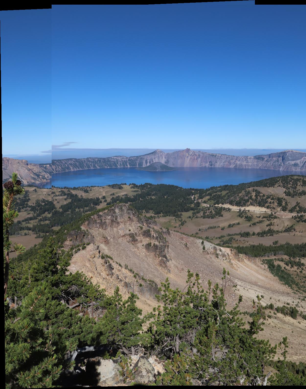
Finally, you can see the results of using the automatic feature method vs the manual one.
Auto

Manual
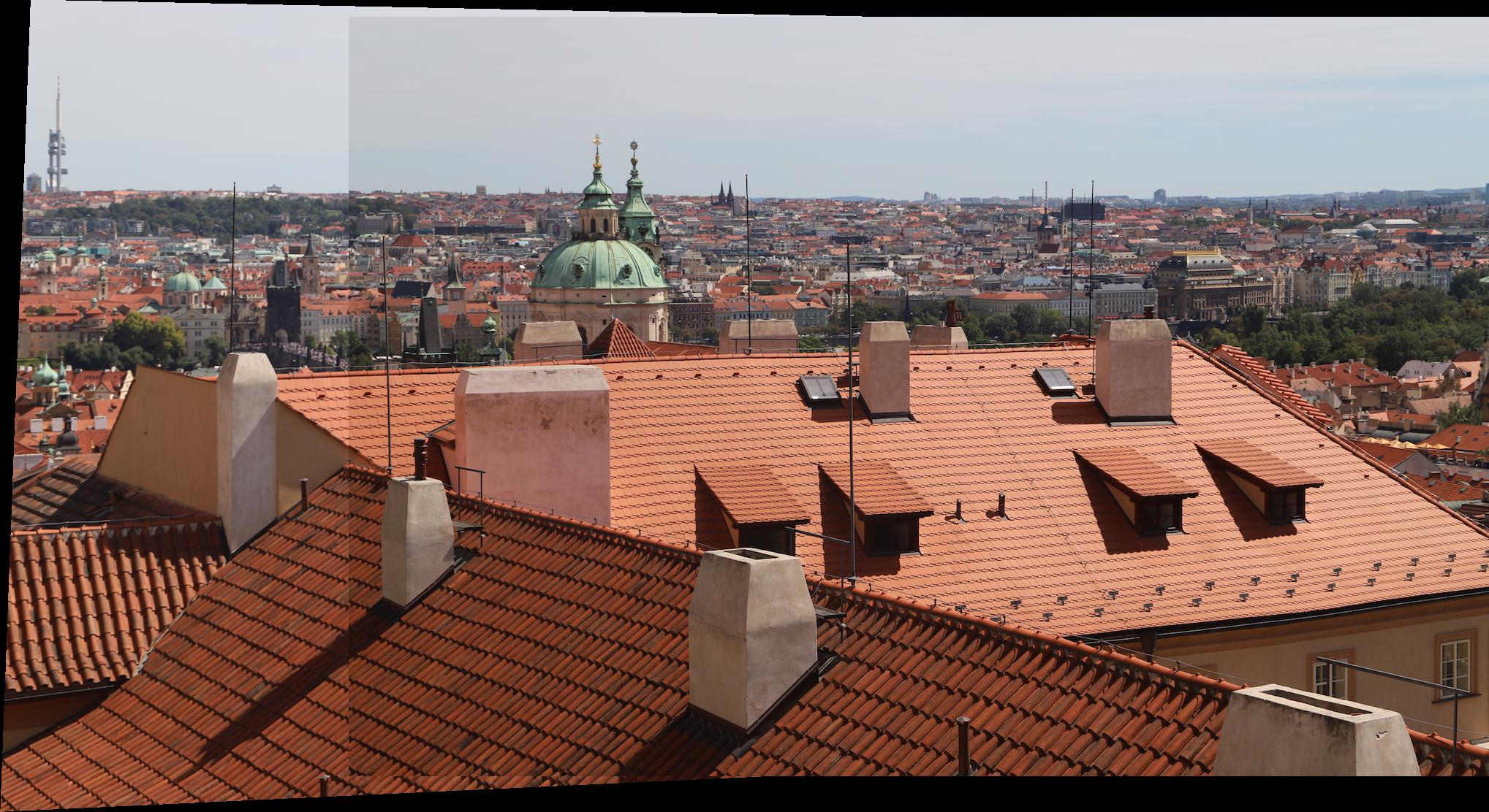
Auto
Manual
Auto
Manual
Conclusions
This was a very cool project. It was fascinating to see how simple linear algebra is enough to get some pretty impressive results. It was also a valuable experience to read a research paper and implement the algorithms described, especially since I had to really understand what it was saying to do it correctly. I will definitely be using this code in the future for fun and may even improve it!