Violet Yao (cs194-26-afs)
Before we could warp images into alignment, we need to recover the need to recover the parameters of the transformation between each pair of images. In our case, the transformation is a homography: p’=Hp, where H is a 3x3 matrix with 8 degrees of freedom (lower right corner is a scaling factor and can be set to 1). To recover the homography, I collected a set of (p’,p) pairs of corresponding points taken from the two images using ginputs.
\[H = computeH(im1\_pts,im2\_pts)\]
In order to compute the entries in the matrix H, we need to set up a linear system of n equations (i.e. a matrix equation of the form Ah=b where h is a vector holding the 8 unknown entries of H). The system can thus be solved via four or more corresponding pairs.
Now that we know the parameters of the homography, we can go ahead to warp images using this homography.
\[imwarped = warpImage(im,H)\]
where im is the input image to be warped and H is the homography.
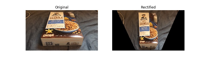
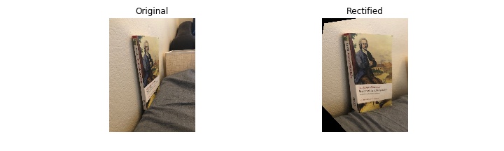
Below are the examples for image rectification! The LHS ones are original images of planar surface and the RHS are those warped to frontal-parallel.
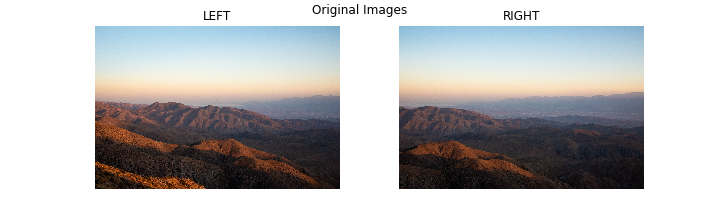
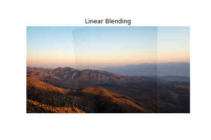
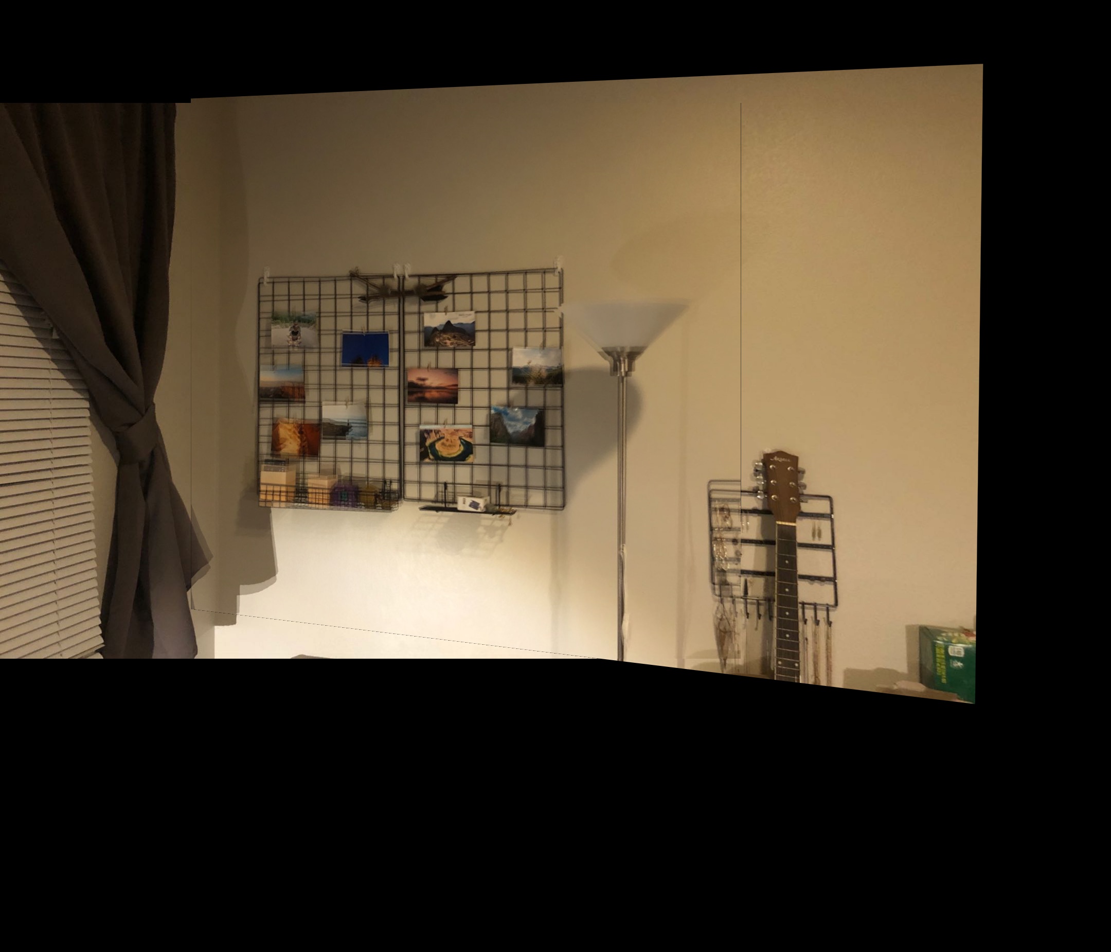
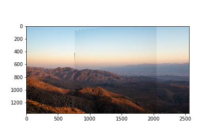
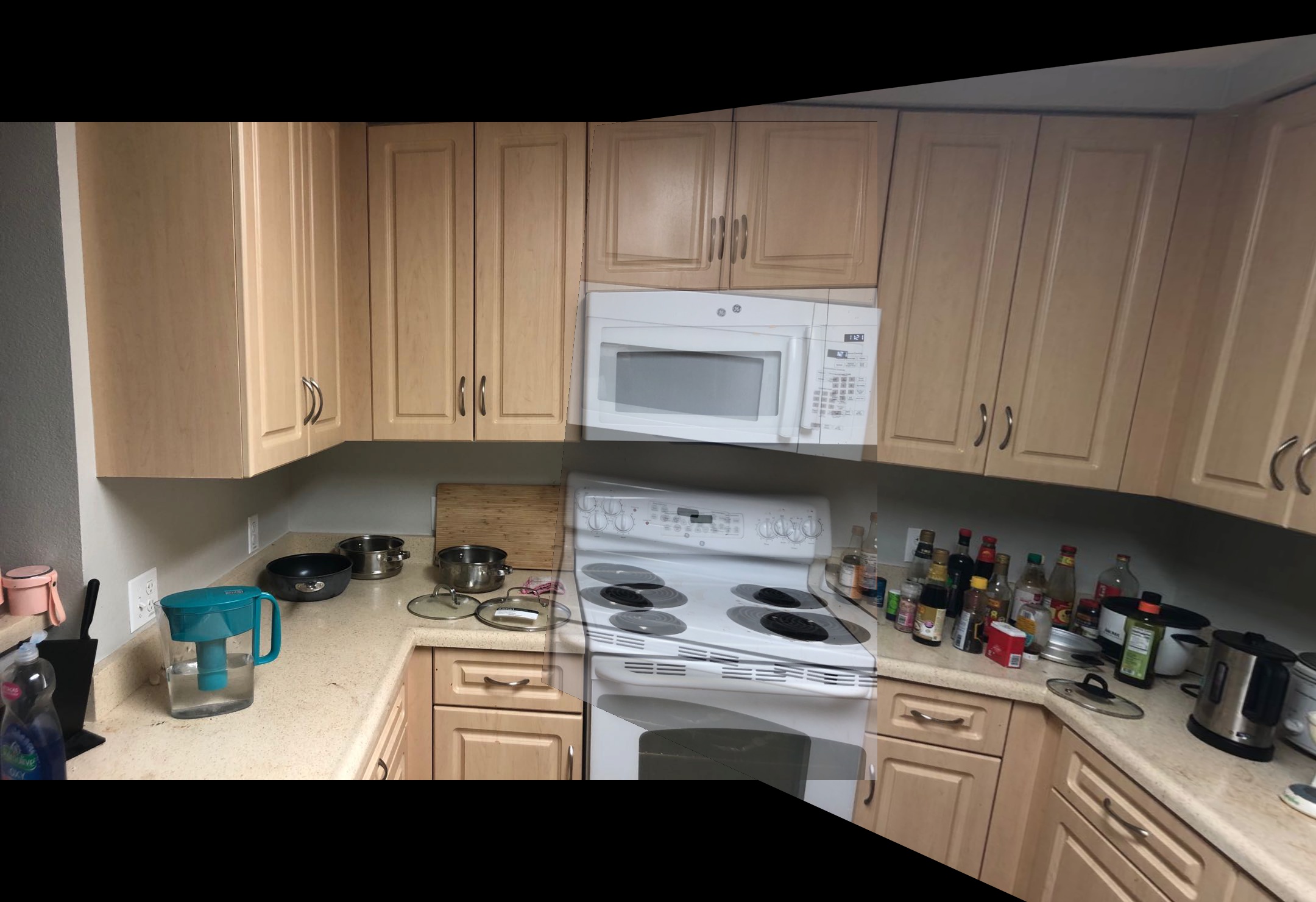
In this part, I warp two images taken at the Grand Canyon so they're registered and create an image mosaic. Instead of having one picture overwrite the other, which would lead to strong edge artifacts, I used linear blending to make it more seamless.
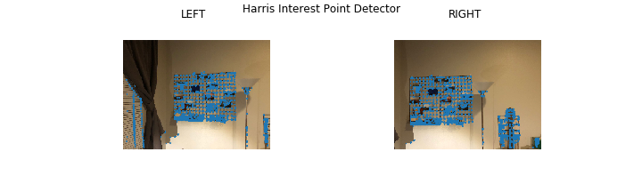
We use harris interest point detector, which is based on change of intensity when shifting a window to all directions, to automatically detect corners in the image. For left & right image below, I plot the top 2000 detected corners for each.
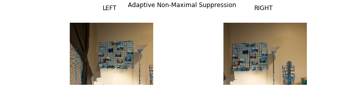
Harris interest point detector returns a large number of points and many of them are clustered together. To improve upon this, we utilize Adaptive Non-Maximal Suppression (ANMS) to reduce the number of points while still keeping the remaining points spreadout. I keep the top 500 points with largest radius.
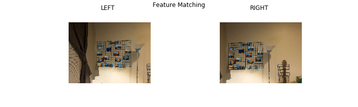
For each point, we extract a 8*8 feature patch from a 40 * 40 window. Then we should normalize the image to zero mean and a standard deviation of 1.
Then, we proceed to match points between the two images by computing squared Euclidean distance between pairs of features (using dist2 from starter code). For each feature, we compute the ratio of best and second best and reject with a threshold of 0.2.
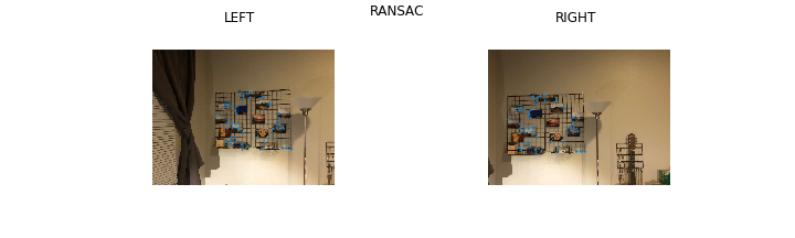
In this step, we select points that will later be used to compute the final estimated homography matrix. Intuitively, good points produce similiar homography. So we iterate 10000 times, choose 4 random feature pairs each iteration, compute homography & use it to warp img1 points to img2 & measure how close they are to true img2 points, set a SSD threshold of 0.5, and keep the feature pairs with the largest number of inliers.
Result from linear blending below:
Manual result from part A:
Auto result from part B:
Additional:
 (It does not perform well since the two only overlaps 20%)
I'm amazed at how similar auto-selected points are to my manually select ones in part A & how well they both perform.