hide forever |
hide once
hide forever |
hide once
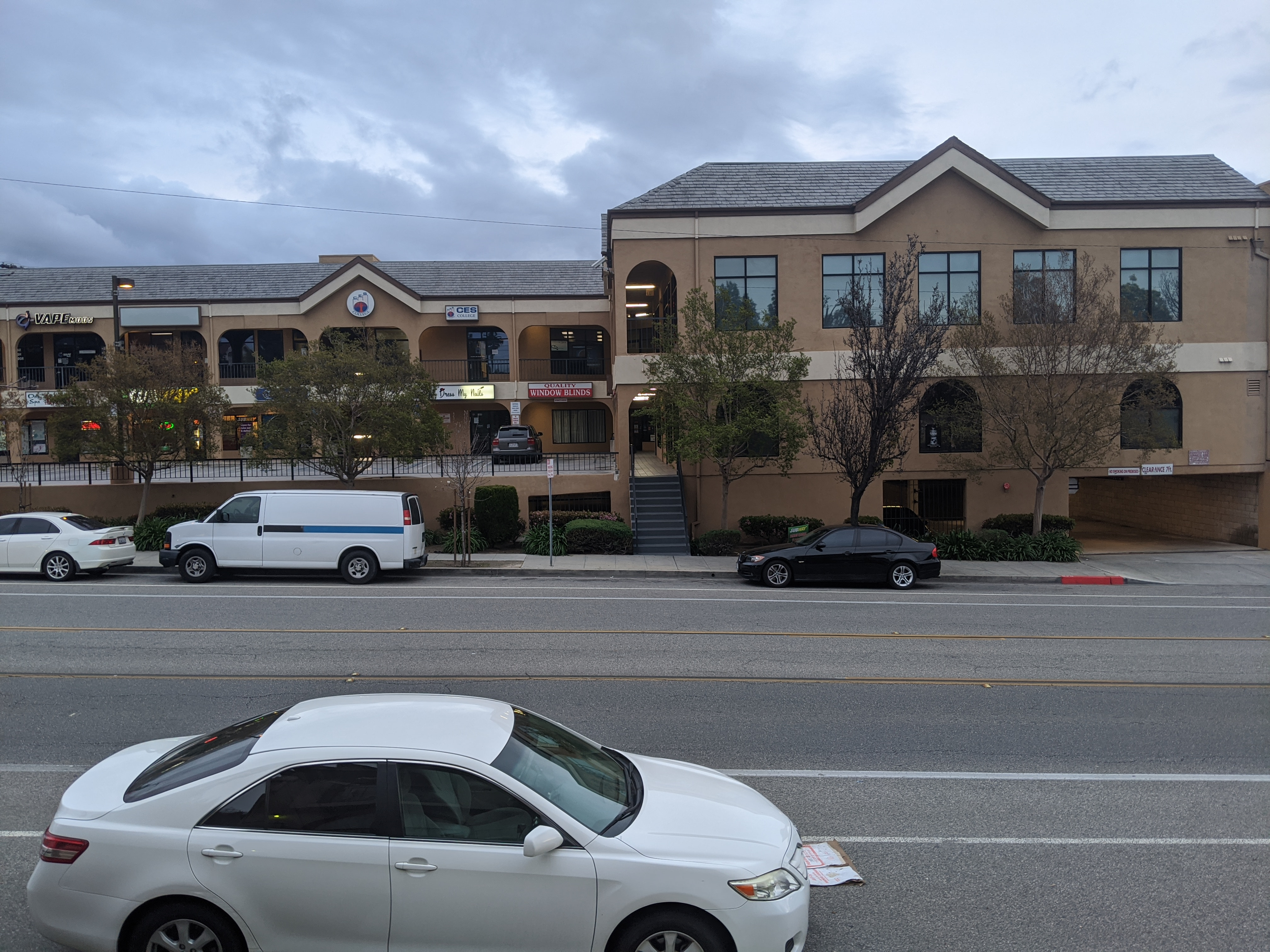
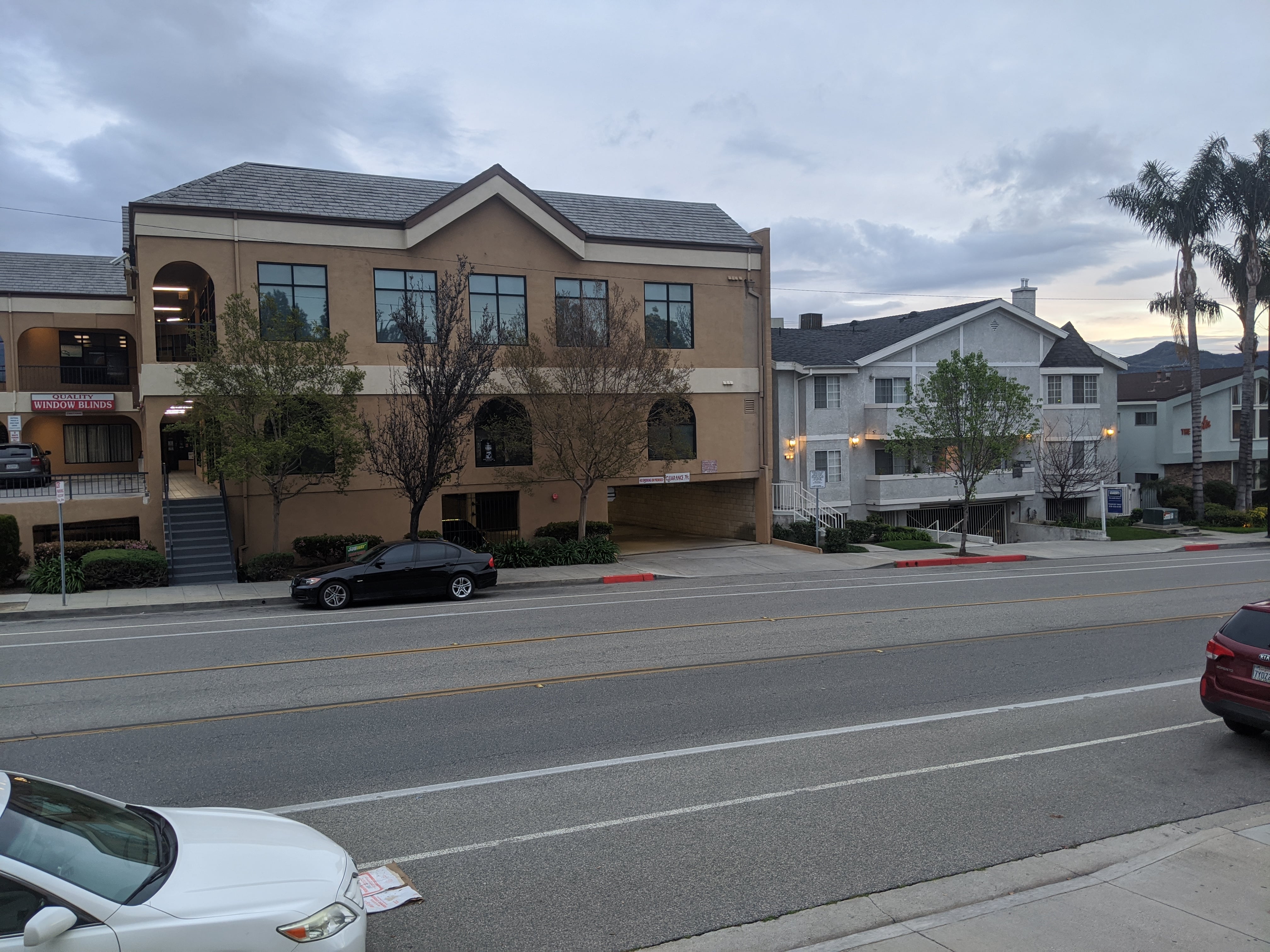
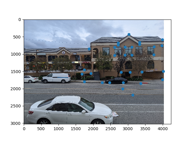
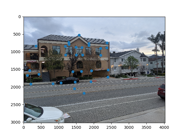
In this project, we capture images that only differ by the rotation angle the image was taken from. We then compute homographies between the images to "stitch" them together. The images used are taken from outside my house in Southern California. additionally, we manually extract 31 correspodning features from each image. These features will be used to compute a homography.
We now need to compute a transformation between the images. Specifically, there is translation and perspective, thus we require a homography.
As setup, we set $$\begin{bmatrix}a & b & c \\ d & e & f \\ g & h & 1 \end{bmatrix} \begin{bmatrix} x_1 \\ y_1 \\ 1 \end{bmatrix} = \begin{bmatrix} wx_2 \\ w y_2 \\ w \end{bmatrix}$$ From this, we can solve for each row $$wx_2 = ax_1 + by_1 + c$$ $$wy_2 = dx_1 + ey_1 + f$$ $$w = gx_1 + h y_1 + 1$$ Expanding \(w\) in the first two equations and then subtracing all but the \(1\) to the other side, we get $$x_2 = ax_1 + by_1 + c - gx_1x_2 - h y_1x_2$$ $$y_2 = dx_1 + ey_1 + f - gx_1y_2 - h y_1 y_2$$ which is linear in our homography parameters. We can then use least squares to solve for the homogrpahy parameters.
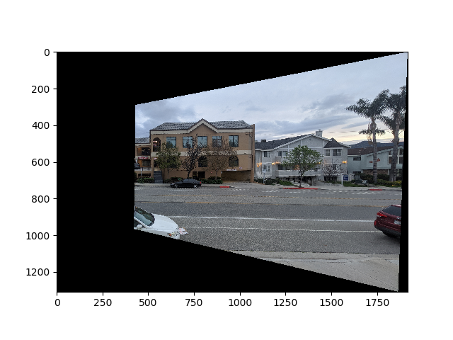
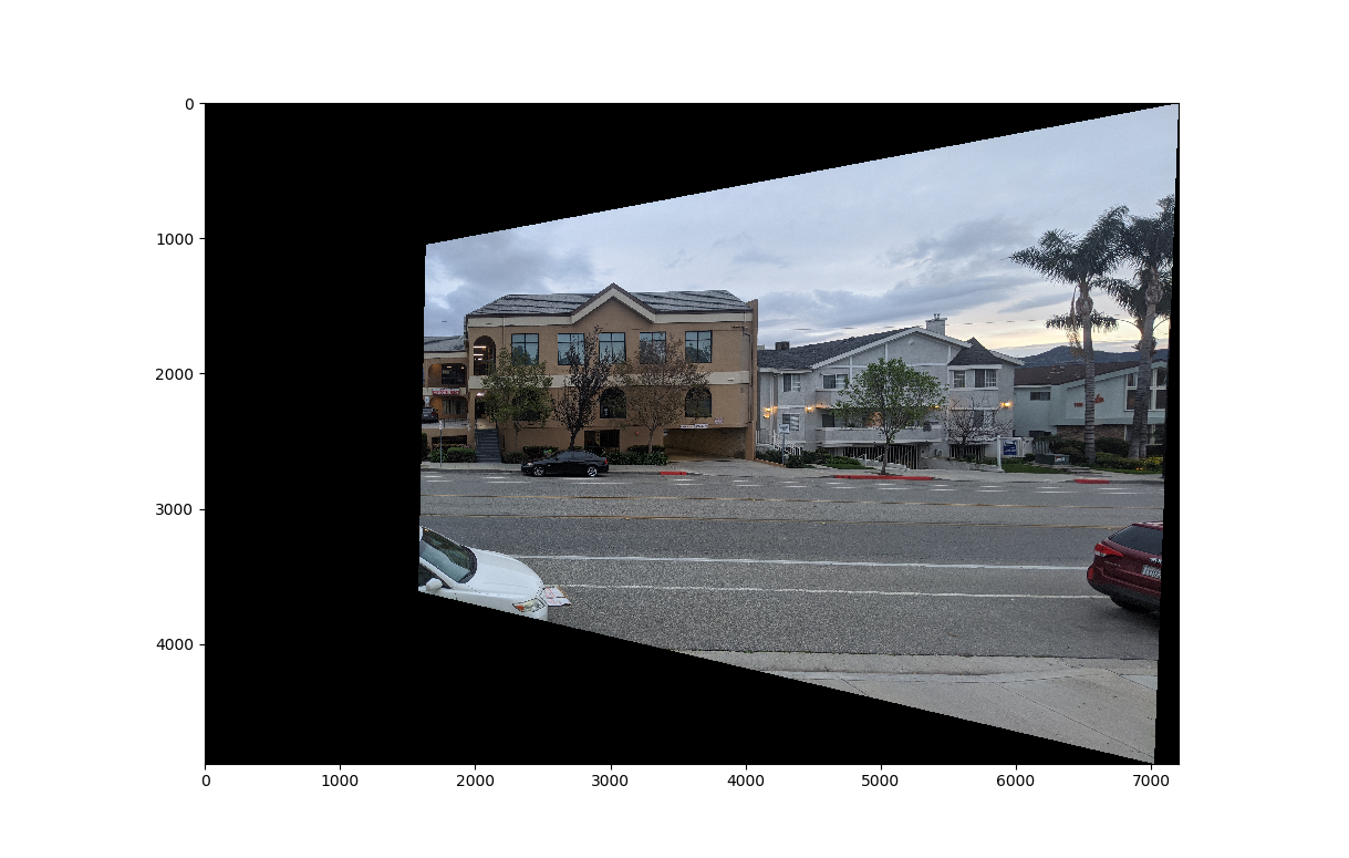
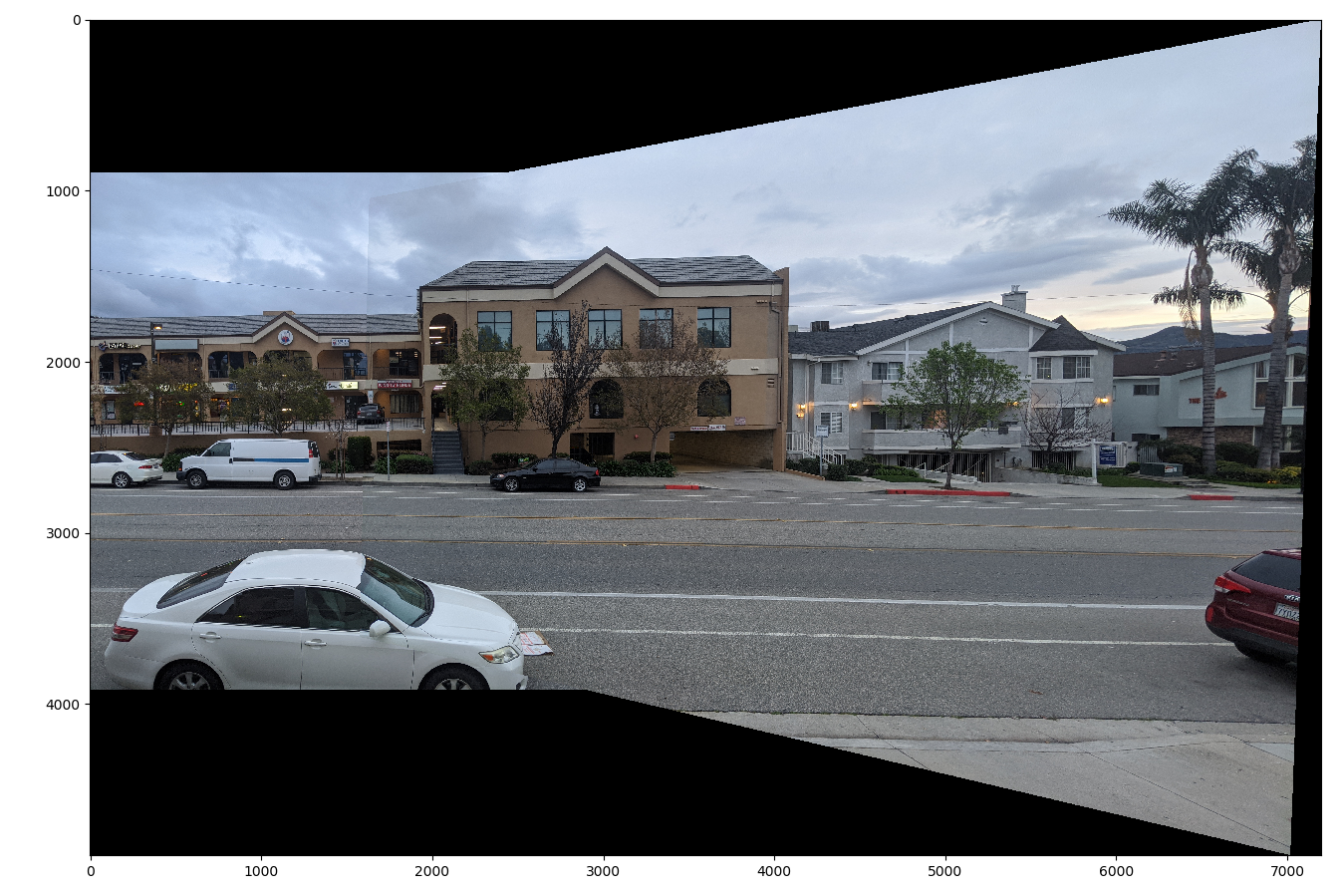
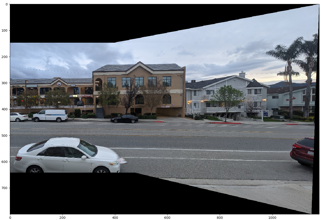
With the homography computed, we have everything we need to warp the image. We warp the right image to align with the left image. This gives us the following result
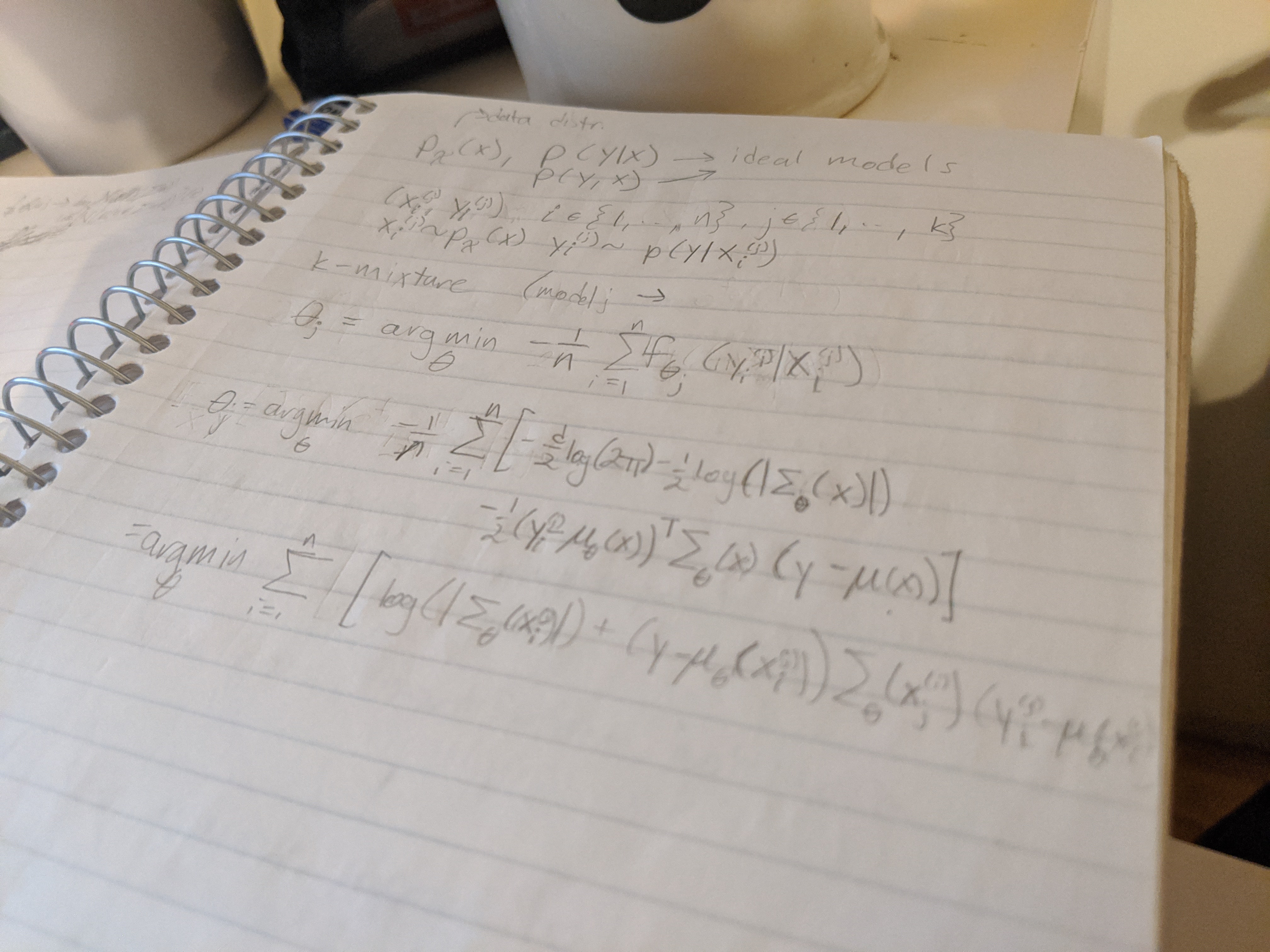
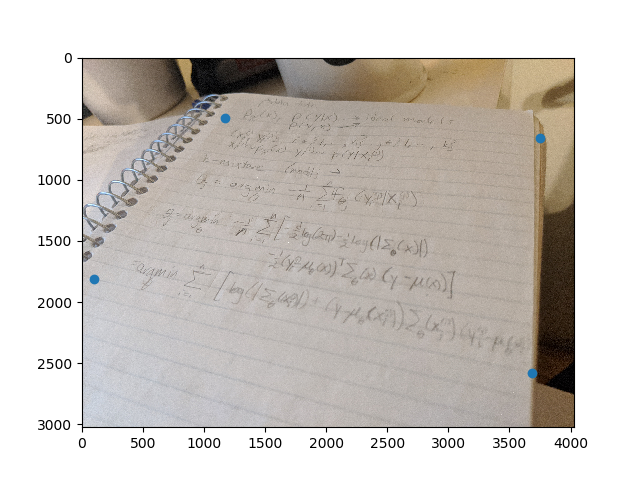
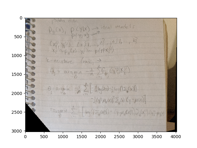
To double check our code, we now test rectification. That is, we take a single image and transform it to changed the persepctive of it. We use a random page from one of my notebooks for this. The features are 4 points chosen from the image, and the transform maps them to a hand picked square.

Before trying anything complicated to stich the images, I first simply overlap them. The warped image is placed on top of the original image. While initially seeming fine, there is an edge artifact on the boundary of the warped image.
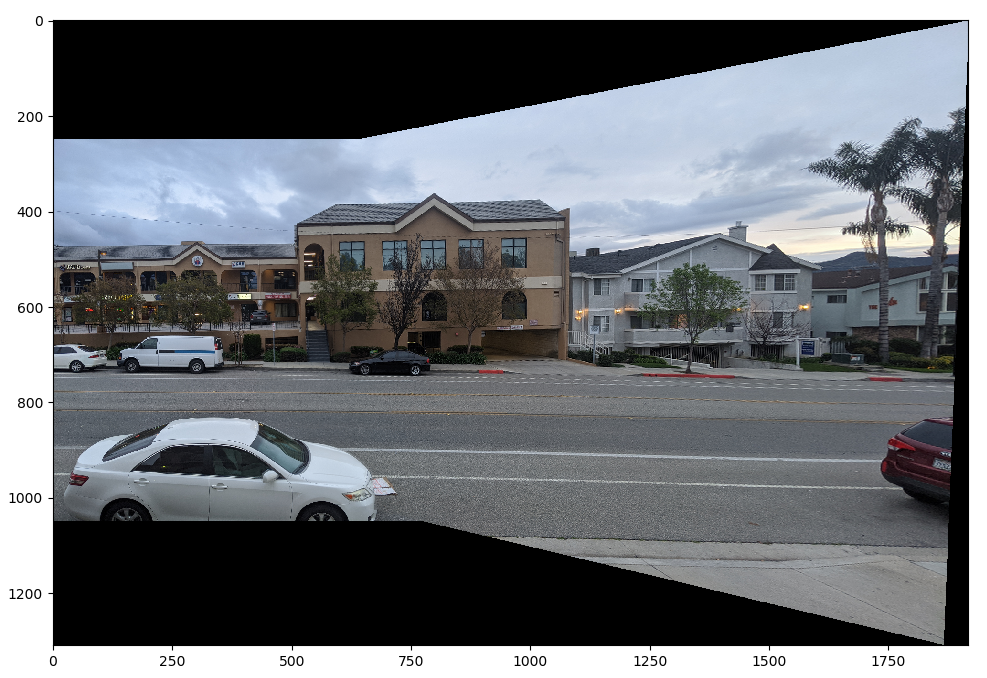
Now we use a Laplacian Stack instead. The first image is a the left image overlayed ontop of the warped image. Then the second image is warped right image overlayed on the left image. The mask is initially set to be one in the warped image, and 0 elsewhere. Then teh boundary in the mask is set to linearly fade off. This gives a much more seamless mosaic, but leaves artifacts where the images disagree, such as on the white car.
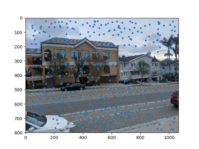
Now that the algorithm works with manually selected points, automate the feature detection to form a fully automated image stitching system. First, we use the Harris Intereset Point Detection algorithm to find Harris Corner points in the images. We use the provided code for this. As you can see, the detected points are very dense.
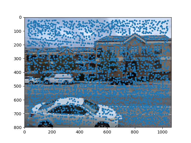
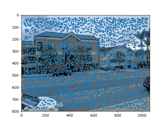
To reduce the number of points while keeping the strongest features and having them spread out, we use Adaptive Non-Maximal Suppression. We limit it to 500 points. As can be seen, the points are far more sparse and are uniform over each image.
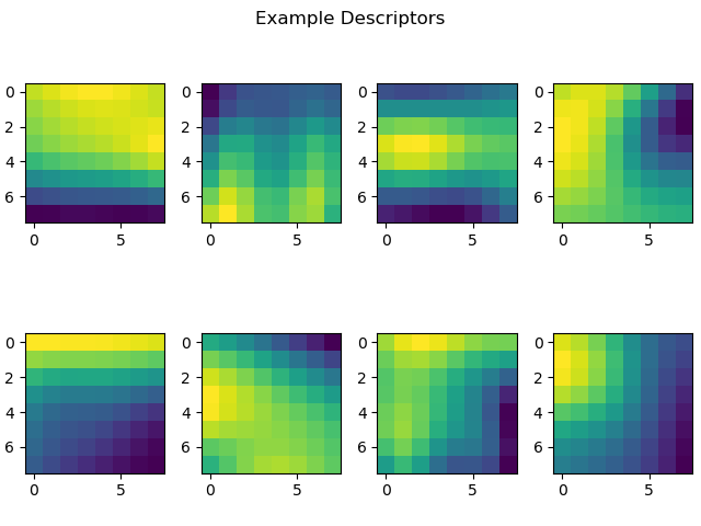
Now that we have a list of candidate points, we require a way to match them. To do this, we extract feature descriptors for each point. The feature descriptor is taken by low-passing the image, then taking 40x40 grids around each pixel and subsampling it to 8x8 (hence the low-pass to prevent aliasing). Each descriptor is then normalized (mean subtracted and standard deviation divided). It is worth noting that an even kernel size would allow a .5 group delay, and thus allow for perfectly aligning each descriptor with the point in the middle, but cv2 does not allow for even kernel sizes. However, we remain consisten with the allignment so this is not an issue, there is just .5 sample shift in the descriptors.
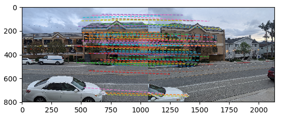
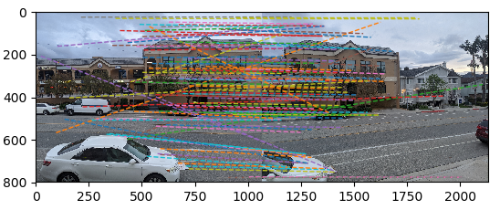
With feature descriptors, we can now match features between images. To do this, we first simply calculate the l2 distance between features from the first image to the second image. The candidate match for each feature in the first image is the one in the second image that minimizes the l2 distance of the descriptors. However, these are very noisy weith several false matches (not all features are present in both images). To filter out the false positives, we compare the score of the second best match. For a specific feature in the first image, if the ratio between the distance to the best match and distance to the second best match in the second image is above a set threshold, we decide that this is a false positive. I set this threshold to .5, which reduces the number of mathces down to 101.
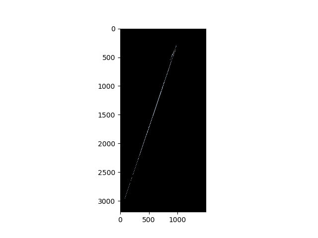
While these matches are fairly well formed, there are several outliers. If we try and find the hmography map and form the warped image, we get an monstrous result due to the outliers.
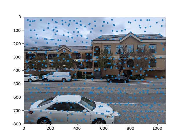
To rectify this, we wish to get rid of outliers. For this, we run the RANSAC algorithm. We set the maximum distance for an inlier to 10, and set the minimum nuber of iterations to 100. This narrows down 65 features. As can be seen we get much better results, and our resulting mosaic is nearly the same as with hand-picked features.