Part A: Image Warping and Mosaicing

Recovering Homographies

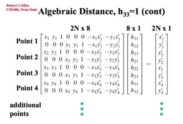
Our first objective was to recover the homography matrix, which defines the transformation between a pair of images. In our case, we want to find the transformation between our original input and our desired rectified output shape. To recover the matrix, we choose multiple correspondence points and solve using least squares.

Rectifying Images

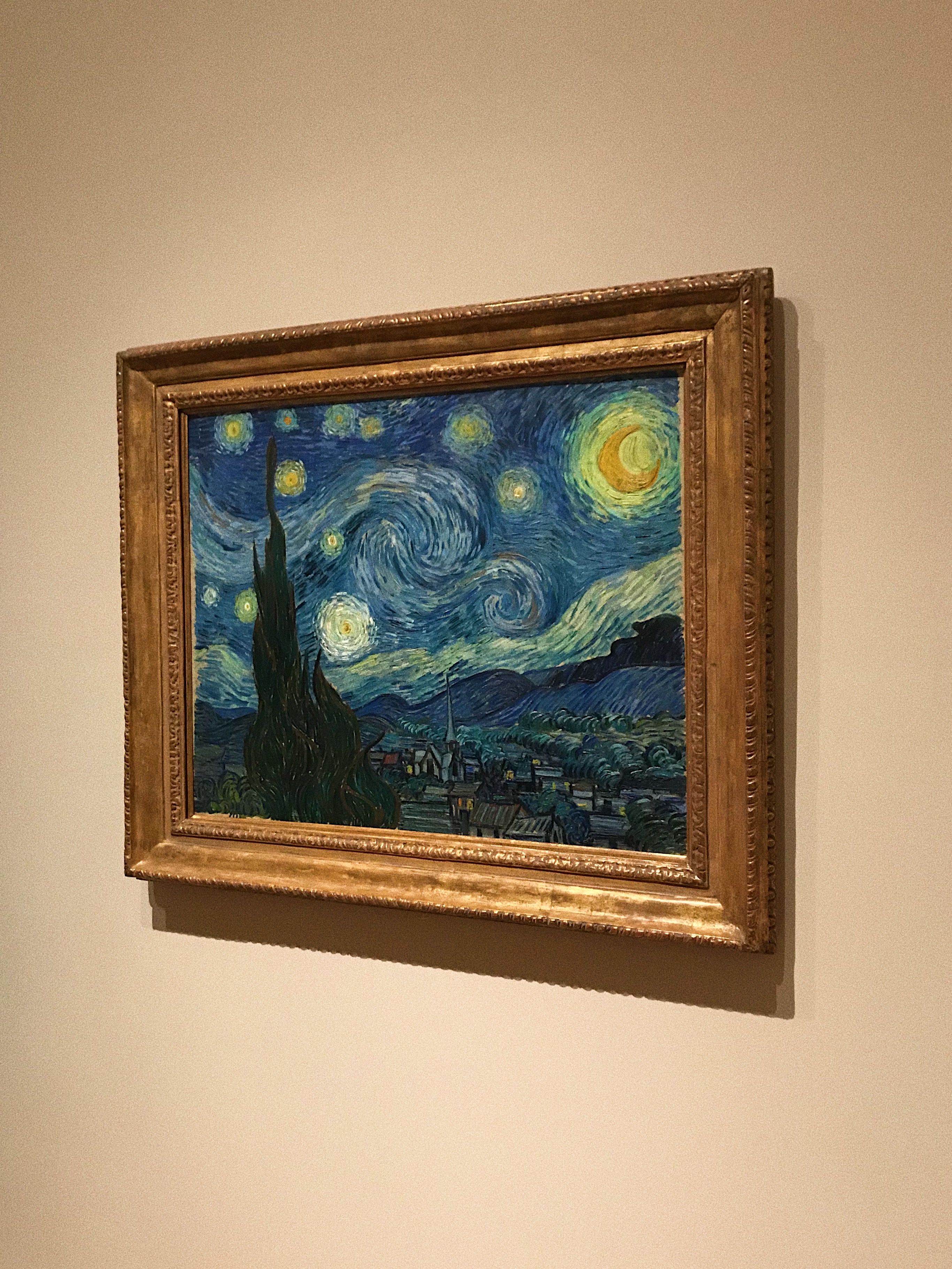
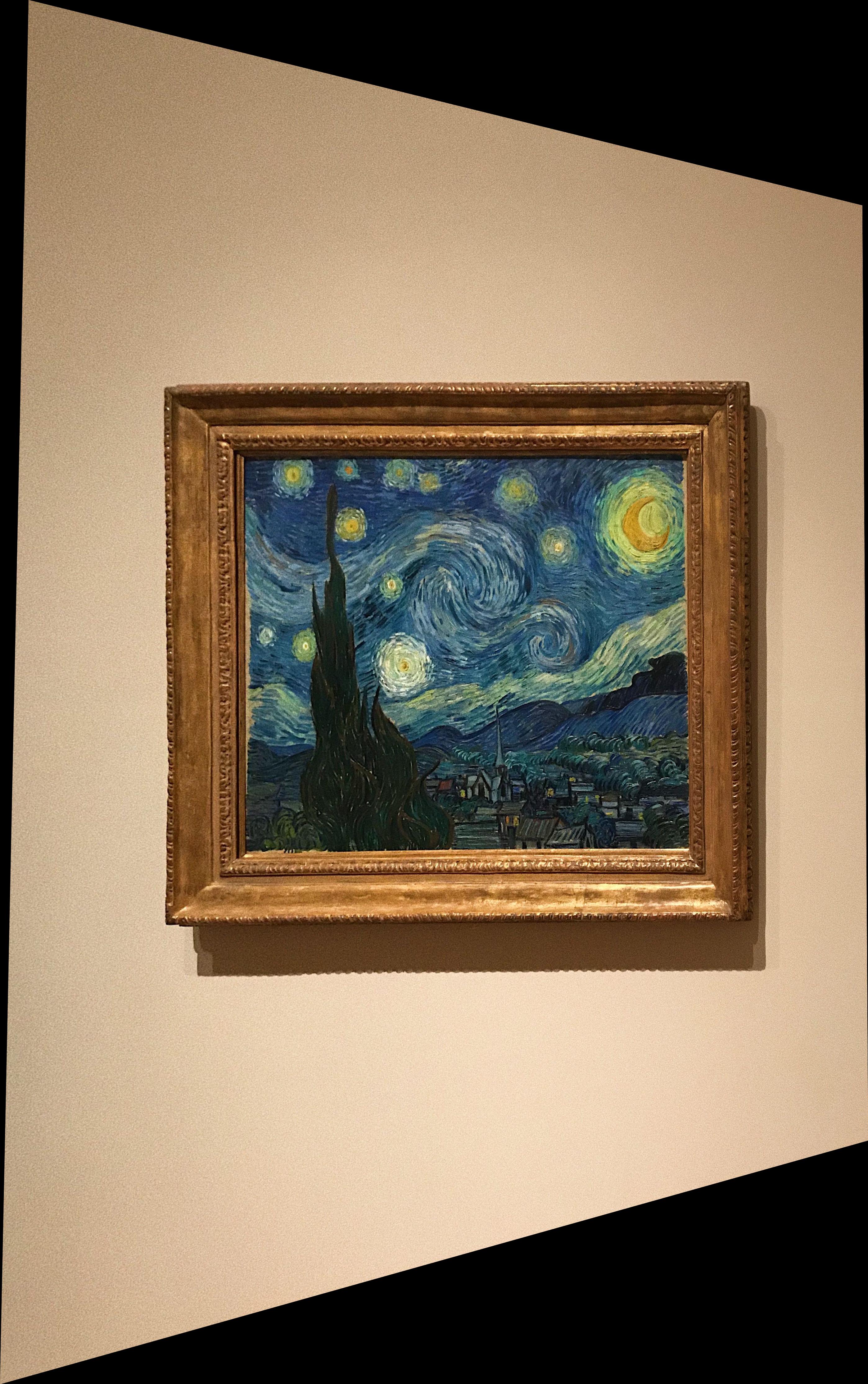
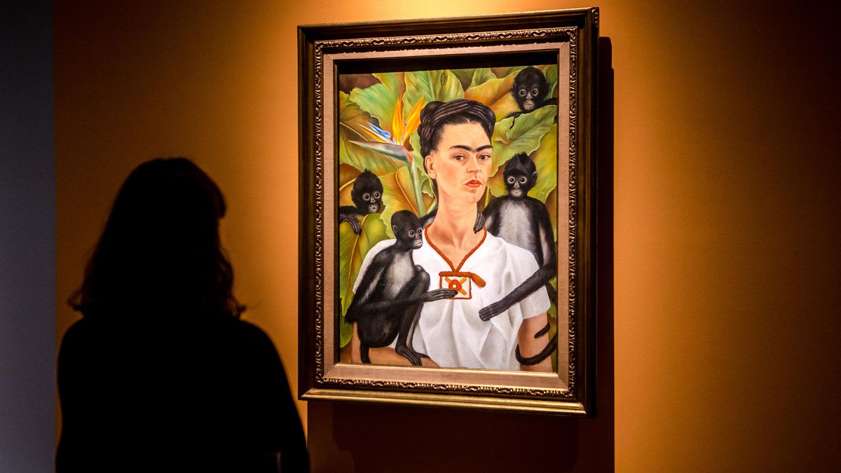
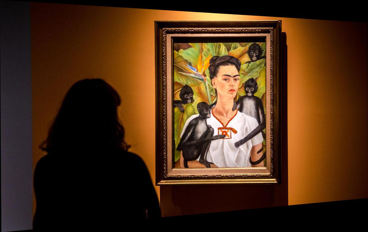
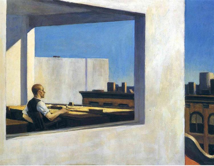
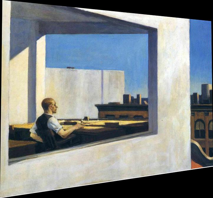
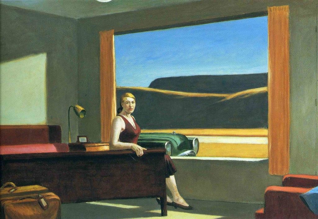
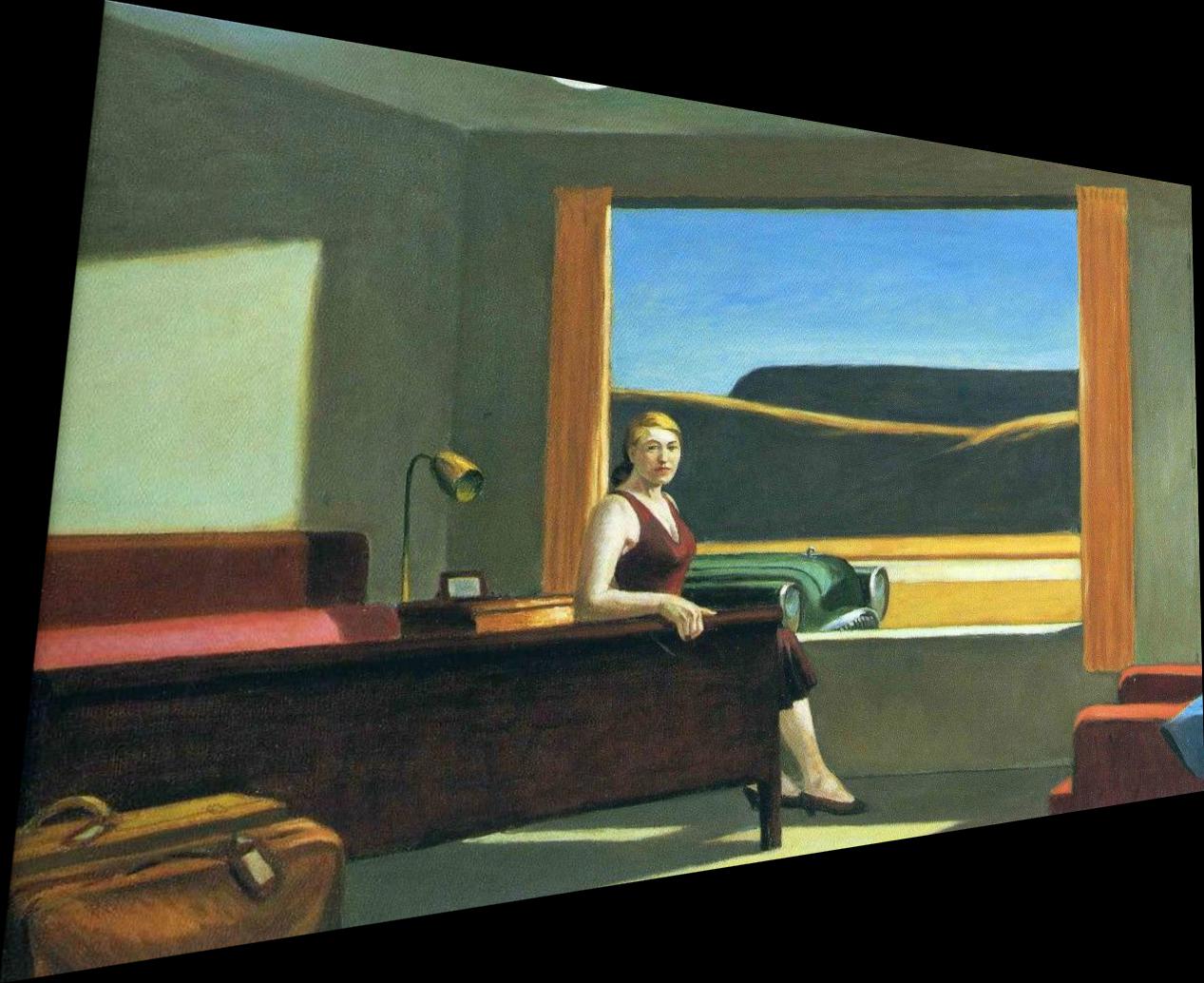
The next step is to rectify the images. The trick here is to find sample images with planar surfaces that can be warped so that the plane is frontal-parallel. The next step is to define the correspondences for our desired output in rectangular coordinates, compute the homography, and warp our image. In my first attempt, I created a bounding box that just displayed all pixels contained within the four corners I chose to rectify. However, after working through part b, my implementation now pipes in corners to find a bounding box for our warped image. Below are some results of rectified artwork. I chose some famous paintings captured at unfortunate angles in an attempt to restore them. In the spirit of self-isolating, I rectified some lonely Edward Hopper paintings which are less lonely but also notably less pretty.

Original Image	Rectified Image
starry night
frida kahlo
office in a small city
western motel

Blending Mosaics (Manually)

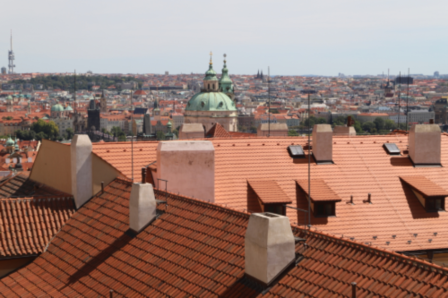
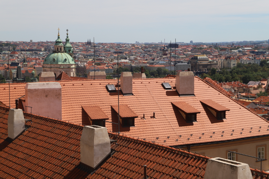
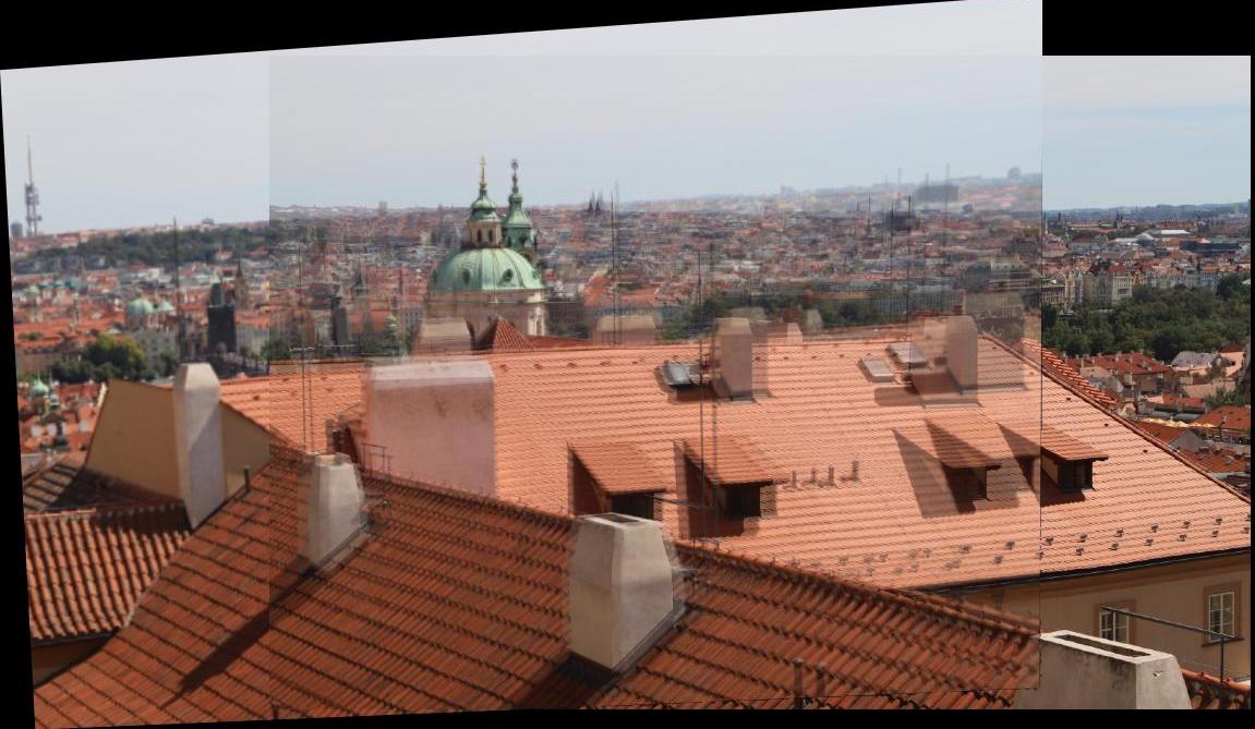
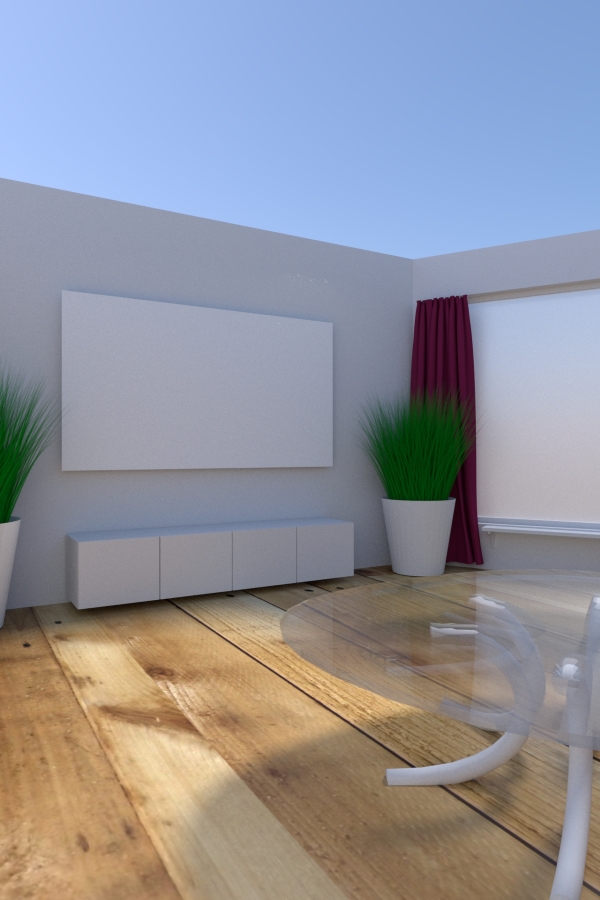
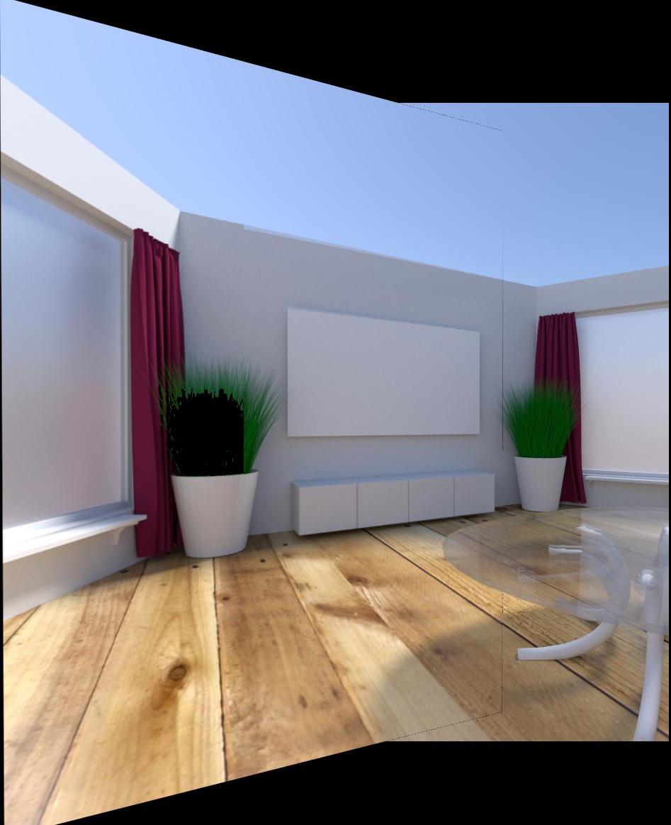
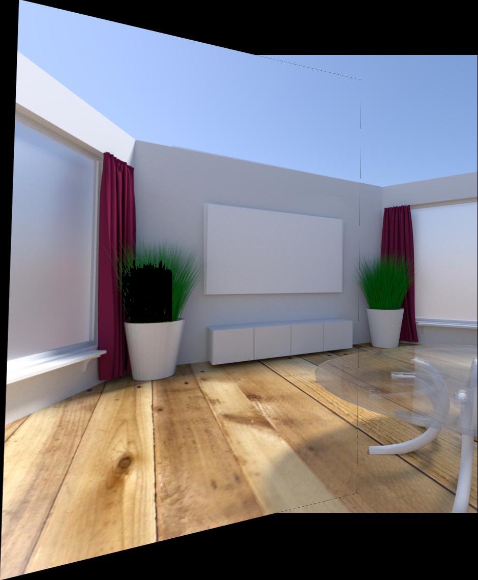
A cool application of image warping is creating panoramas. In order to blend two images together to create a panorama, I first manually defined correspondence points. Using these correspondence points, I can warp one image to the other. After, I blend the two images onto one canvas. I added an alpha channel, and adjusted the values for the unwarped image in our overlap region in order to create a more seamless blend. The city rooftops and lake images are course provided images, and the blender-rendered room image is from the Computer Vision Lab at Linköping University. As we can see in the resulting mosaics below, the images aren't quite as aligned as we'd hope. In the next section, we'll explore methods of improving our technique.

Left Image	Right Image	Mosaic Image
city rooftops
lake
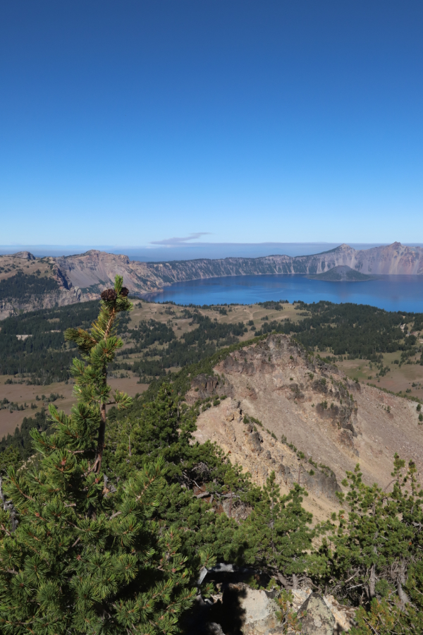
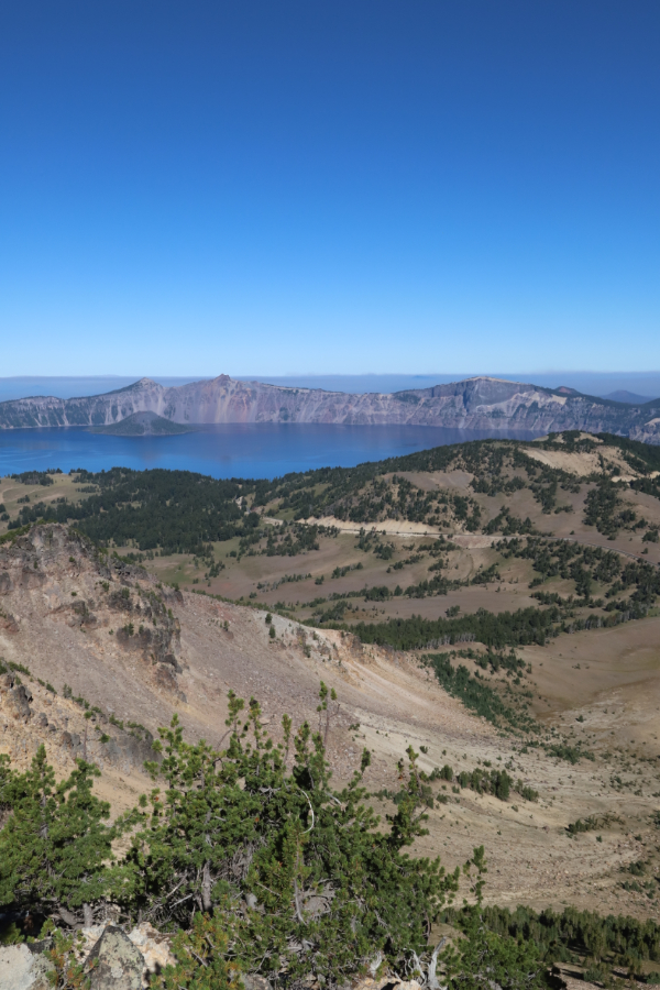
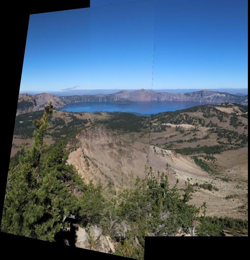
blender room

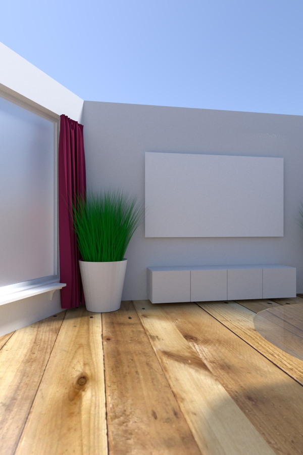
Reflection for Part A

Although I've been stuck inside, I was able to have fun with the images I tried rectifying. It was interesting to test out different artwork with varying results.

Part B: Feature Matching for Autostitching

Now, let's explore an easier method of image mosaicing! Instead of picking correspondence points manually, we can automate this process by implementing the procedure described in “Multi-Image Matching using Multi-Scale Oriented Patches” by Brown et al. I simplify the procedure by using single-scale matching instead of multi-scale.

Detecting Corner Features

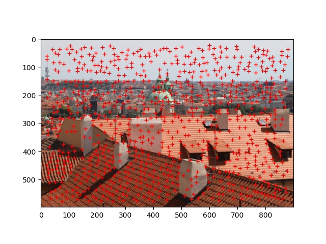
Our first step is to find correspondence points in our images that may help us match. The idea is to find "corner" points with high detail and variation around the area, as opposed to a less descript point that cannot be easily matched. In the image below, the red points illustrate the corners found by the course-provided harris corner algorithm. As you can see, the algorithm returns various corners that we don't necessarily need.

Adaptive Non-Maximal Suppression

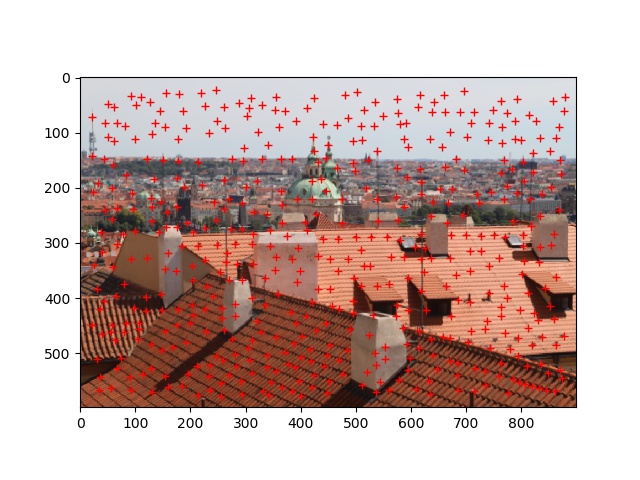
I filtered the number of corners by implementing ANMS. The function sorts harris corners by their strength value, calculates the distances between all corners, finds a minimum suppression radius for each corner, and keeps the corners with the highest minimum suppression radiuses. As shown in the images below, the number of corners and their distribution has improved.

Image	Harris Points	ANMS Points
city rooftops

Extracting Feature Descriptors

Using our ANMS corners, I extracted a feature descriptor for each corner. This involved extracting a 40x40 patch centered around an ANMS corner. I then downsampled the patch to 8x8 and normalized.

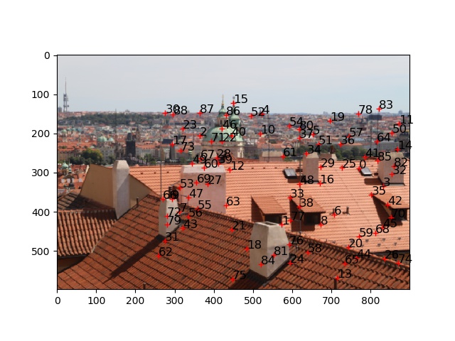
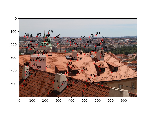
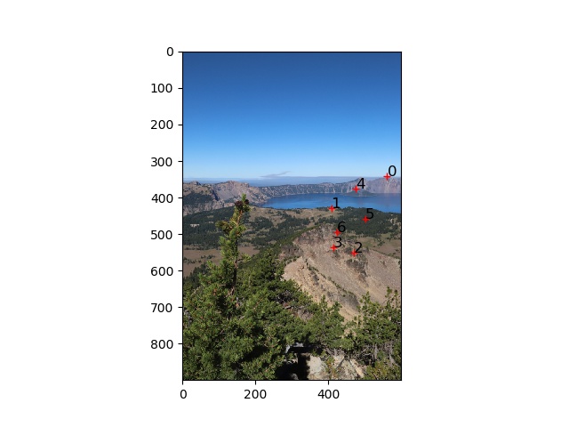
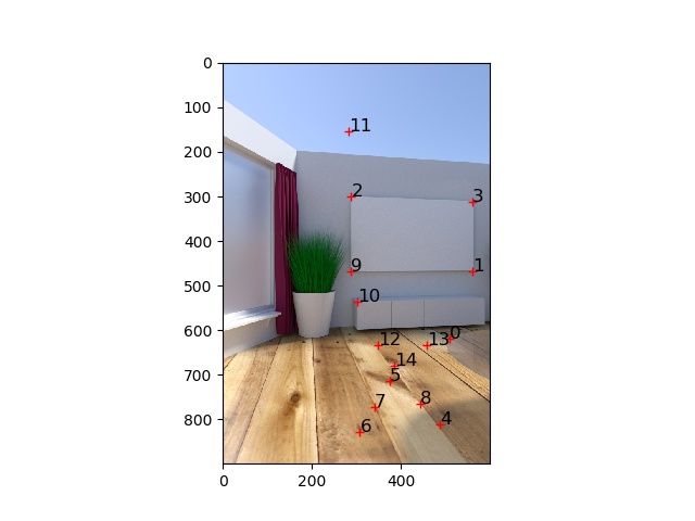
Matching Feature Descriptors

After extracting feature descriptors for the two images being mosaiced, we want to match these descriptors. Using the dist2 function provided, I calculated the distance between my two feature descriptor arrays. I then used the top two matches in the resulting array to calculate a ratio using Lowe thresholding. If the ratio is below the threshold, I kept the pair of points as a valid match. The images below show the resulting matched points.

Image	Left Image Match Points	Right Image Match Points
city rooftops
lake
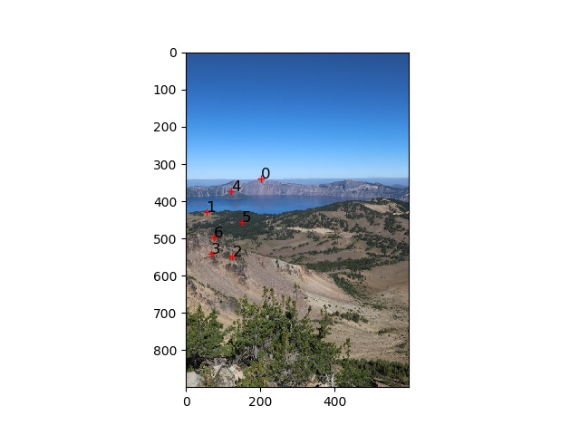
blender room

Computing Homography with RANSAC

Using a robust method like RANSAC helped with computing the best homography for our image warp. To implement RANSAC, I took a random set of 4 matching points and computed the homography using these points. I then transformed the entire first image using this homography matrix and compared the resulting warp with the actual corresponding points in the second image. I kept track of inliers, points with an SSD below a certain threshold. Repeating this process 1000 times, I found the homography matrix with the greatest number of inliers and used this matrix to compute my image warp.

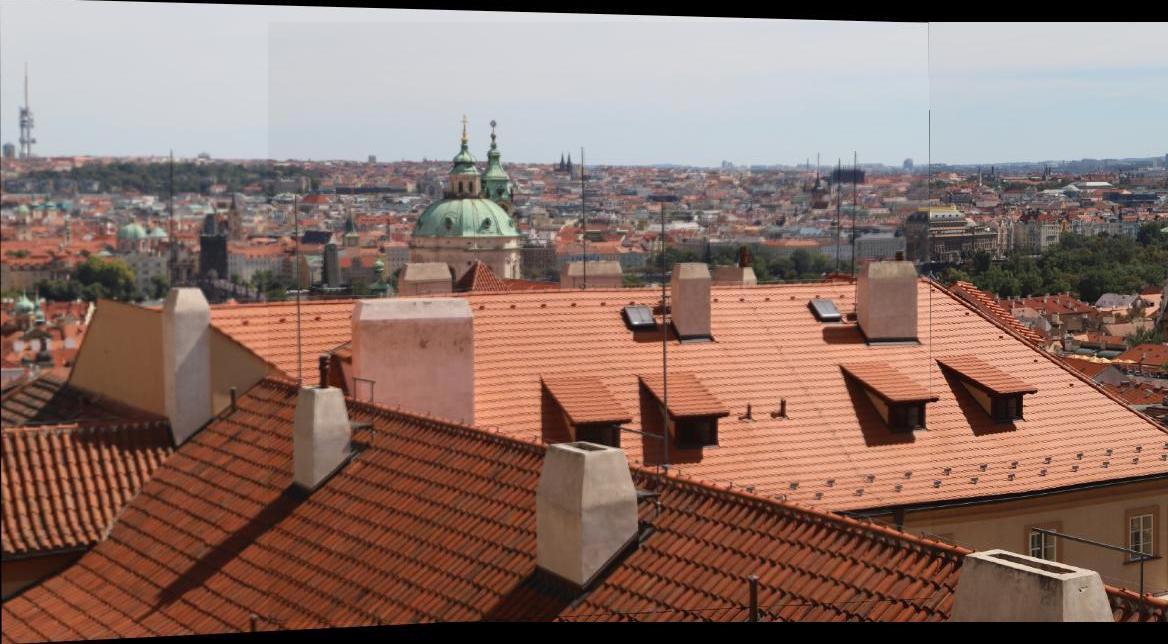
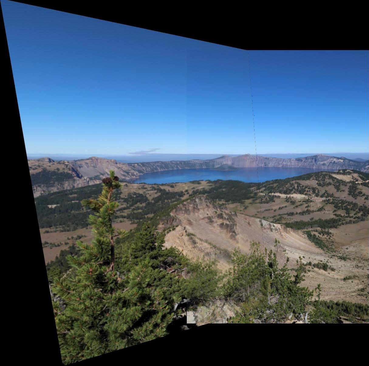
Autostiching Mosaics

Now to the fun part! Using the same mosaic blending function implemented in part a, we autostich our image and compare results! The results are pretty comparable, but autostitching is less work for a better result. I found when working with autostitching that I could improve alignment by changing the min_distance, num_peaks, and whether or not to use ANMS. For example, for city rooftops I actually didn't need ANMS because setting a min_distance=40 and num_peaks=500 yielded a great result already.

Image	Manual Mosaic	Autostitched Mosaic
city rooftops
lake
blender room