Project 5: Autostitching Photo Mosaics
Chelsea Ye, cs194-26-agb
Part 1: Image Warping and Mosaicing
Overview
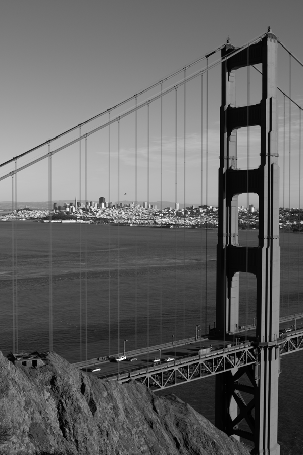
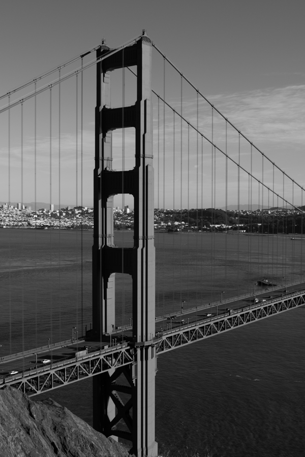
This project is about creating an image mosaic by registering, projective warping, resampling, and compositing photographs that produce a wide-angle view of space. Such photographs must have perspective transformation between themselves, therefore I use photos that were shoot from the same point of view but with different view directions, and with overlapping fields of view.
Recover Homographies
The perspective transformation between each pair of images is a homography:
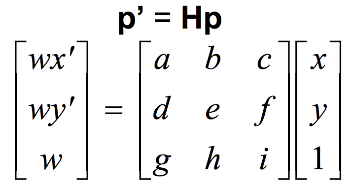
where the 3x3 matrix H has 8 degrees of freedom. We can recover the homography matrix H by taking a set of (p’,p) pairs of corresponding points taken from the two images and setting up a linear system Ah = b using the point pairs. We can solve the linear system using Least Squares:
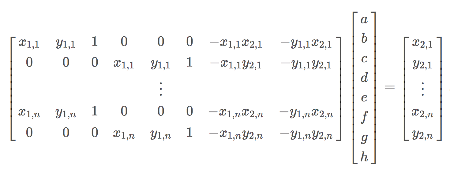
Image Warping and Image Rectification
After recovering the homography, we can now transform our images. Here I perform an inverse warping: for every pixel in the warped result, lookup the corresponding pixel values in the original image by multiply the warped coordinates by the inverse of homography matrix.
We can perform image rectification using the homography to warp images with planar surfaces so that the plane is frontal-parallel. Below I use some photos I took as an example of rectification.
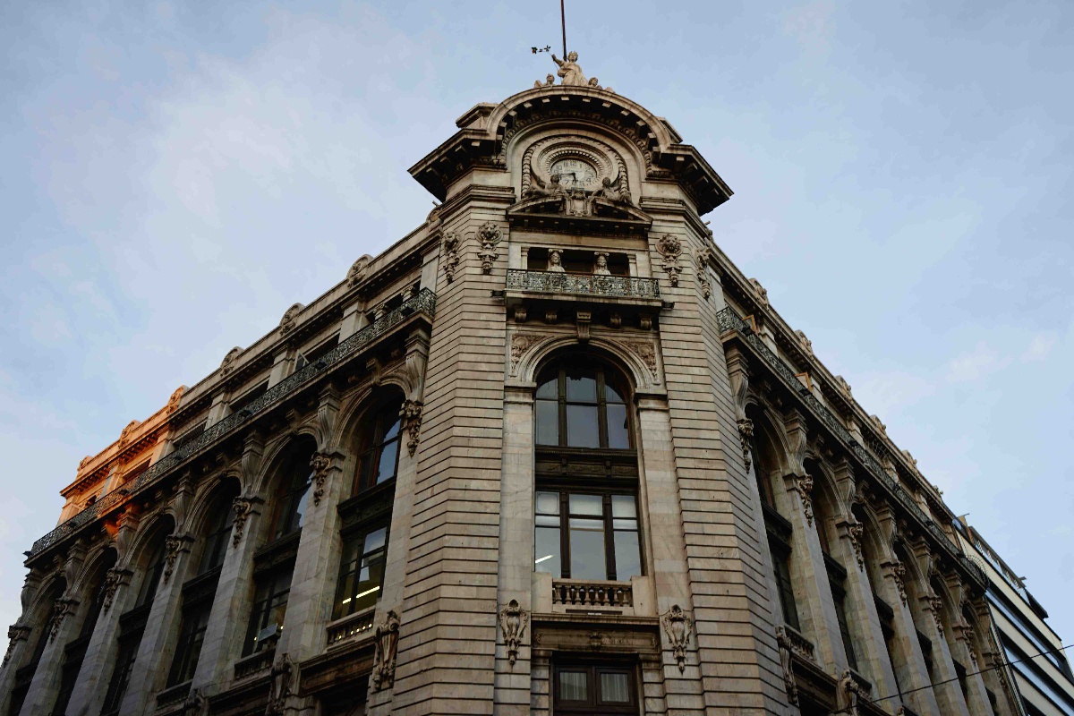
Original Mexican architecture |
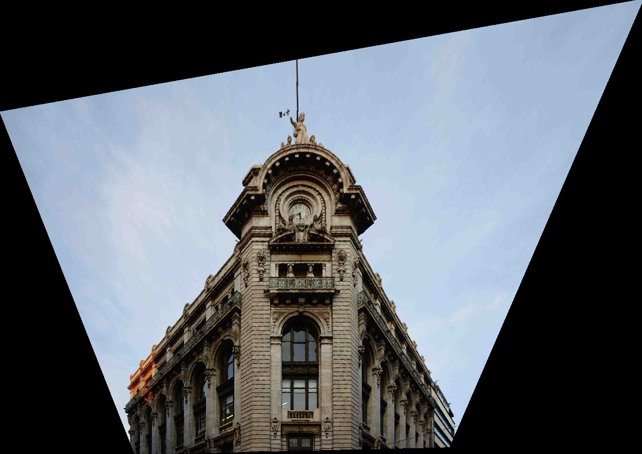
Mexican architecture rectified on the front windows |
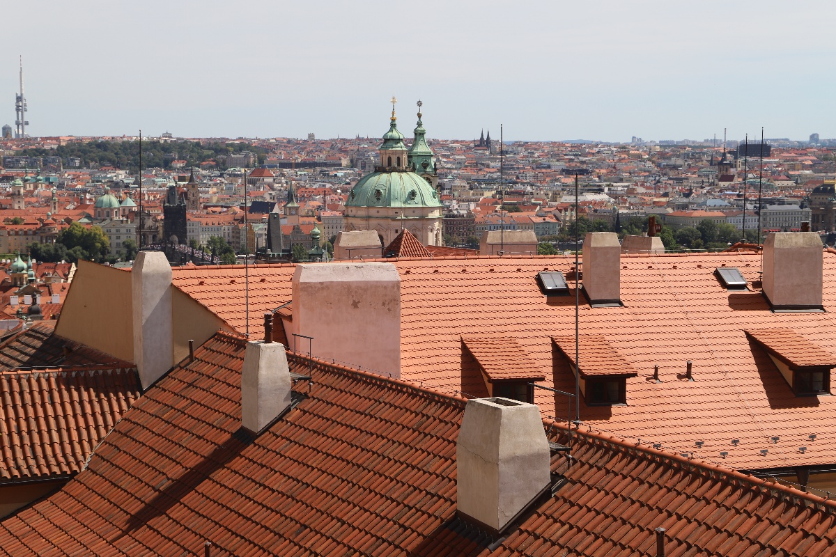
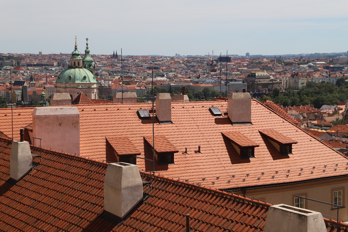
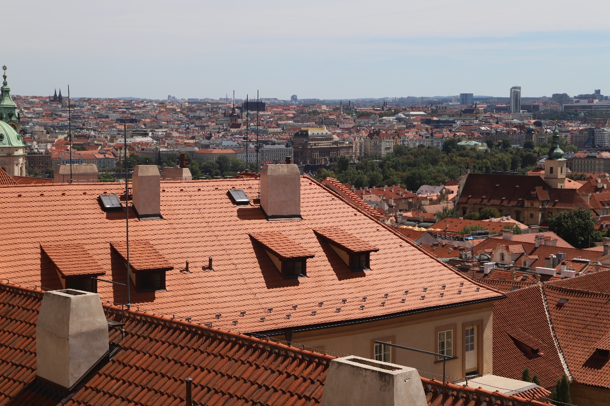
Original Rooftop |
Rectified Rooftop |
Mosaic
With the images warped into one projection, we can now create an image mosaic by blending them together. To smooth the transition between images, I first used a single alpha mask of 0.5 on the overlapping regions. However, the result didn't turn out smooth enough, so I further improved it by making the mask weight fall off linearly from 1 to 0 at the margins (with specified margin width).
Result
|
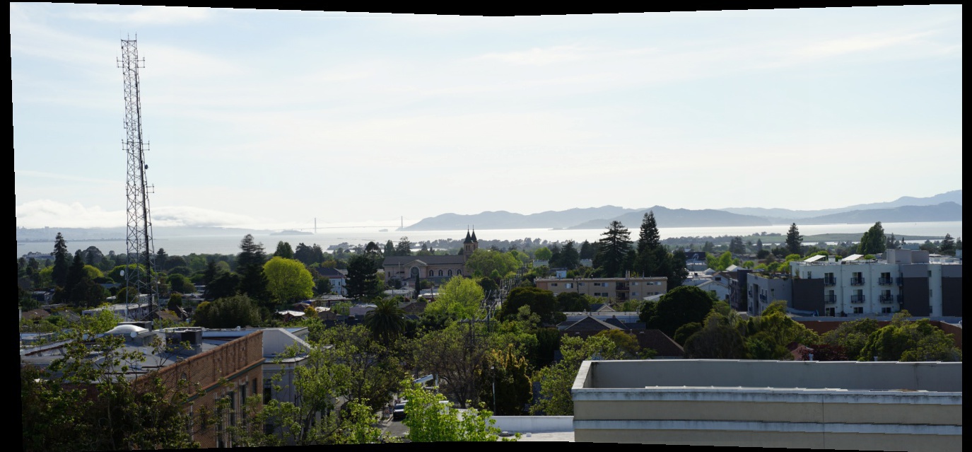
(Course provided images of a city) |
|

City Mosaic |
|
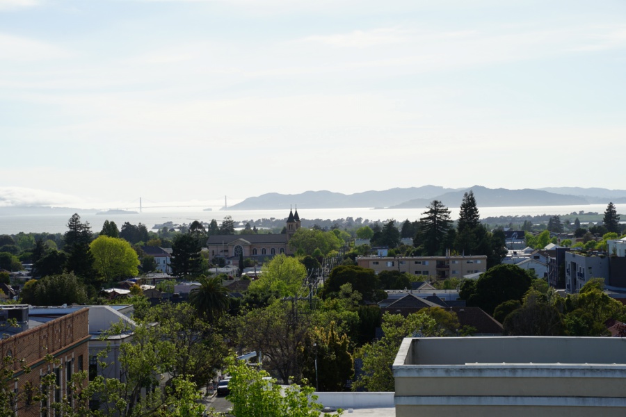
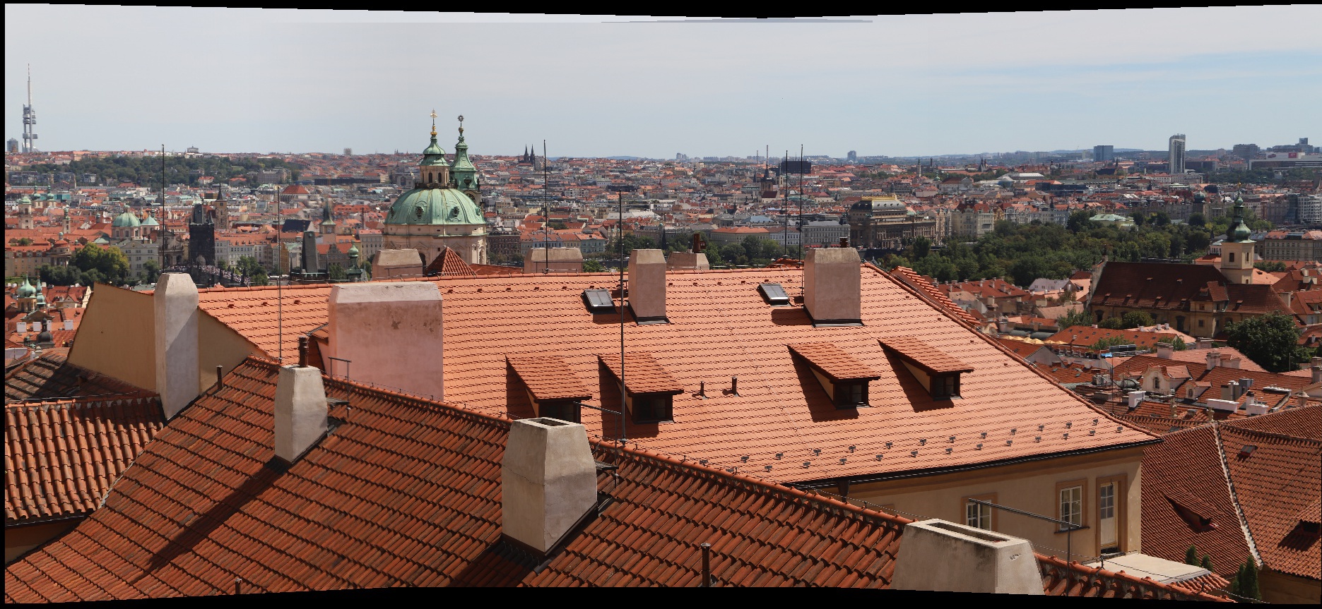
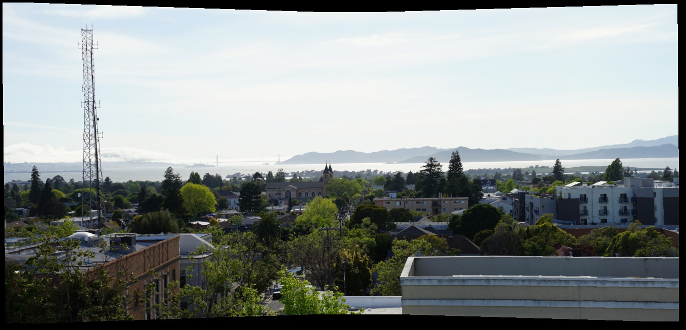
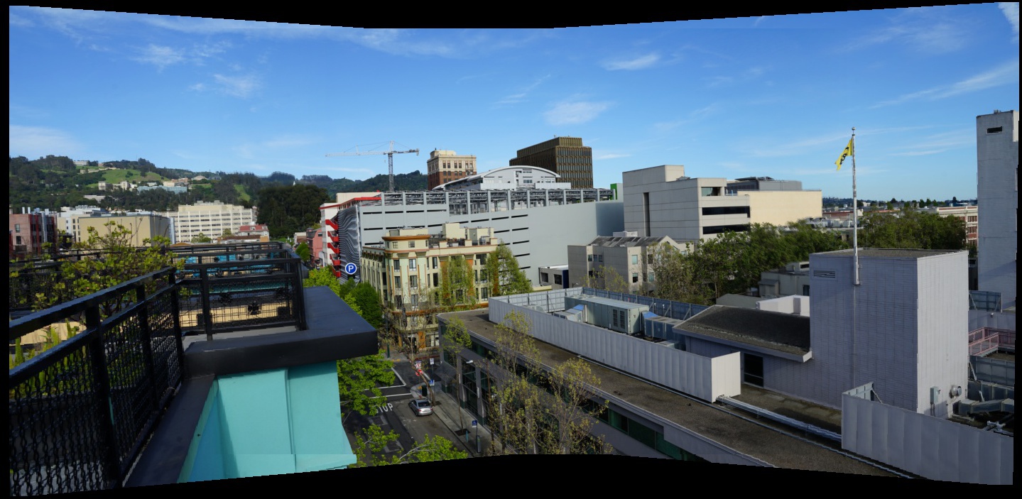
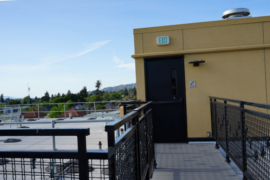
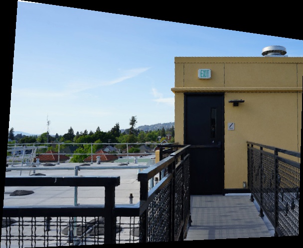
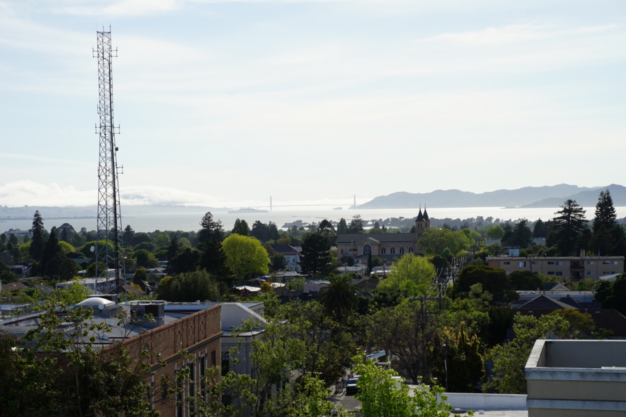
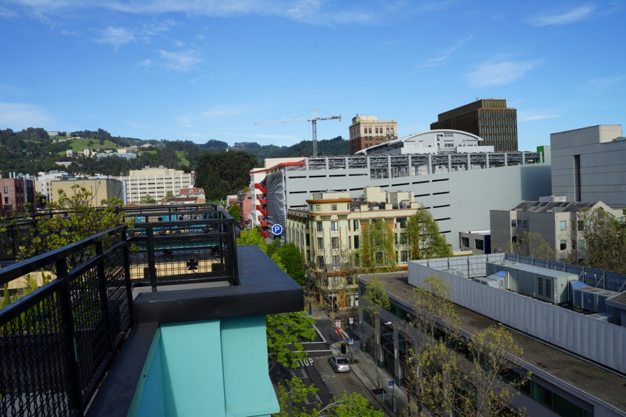
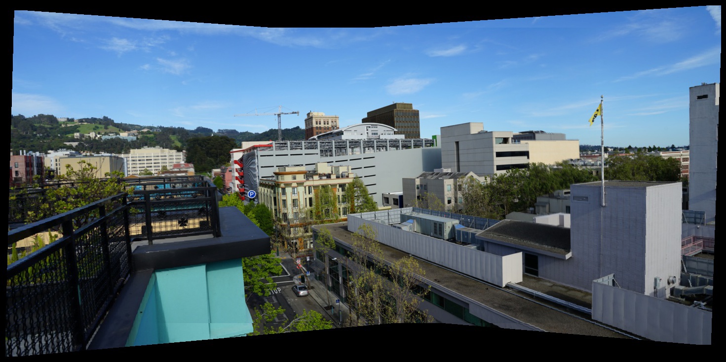
Rooftop view from my apartment |
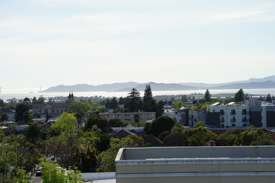
|
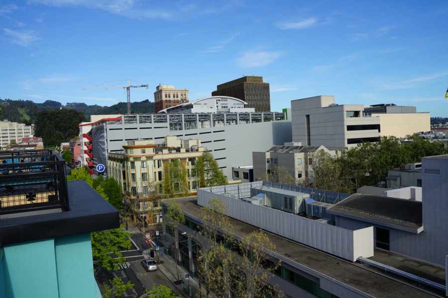
Rooftop view Mosaic |
|
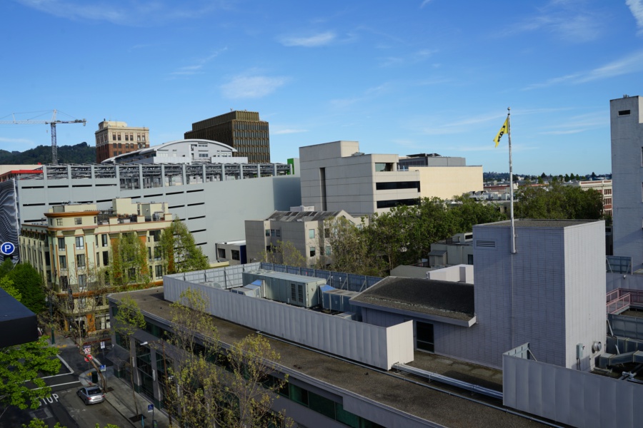
Rooftop view from my apartment |
|
Rooftop view Mosaic |
Part 2: Feature Matching and Autostitching
Overview
Part 2 implements a feature matcher presented in the paper “Multi-Image Matching using Multi-Scale Oriented Patches” by Brown et al. to automate the stitching process.
Harris Interest Point Detector
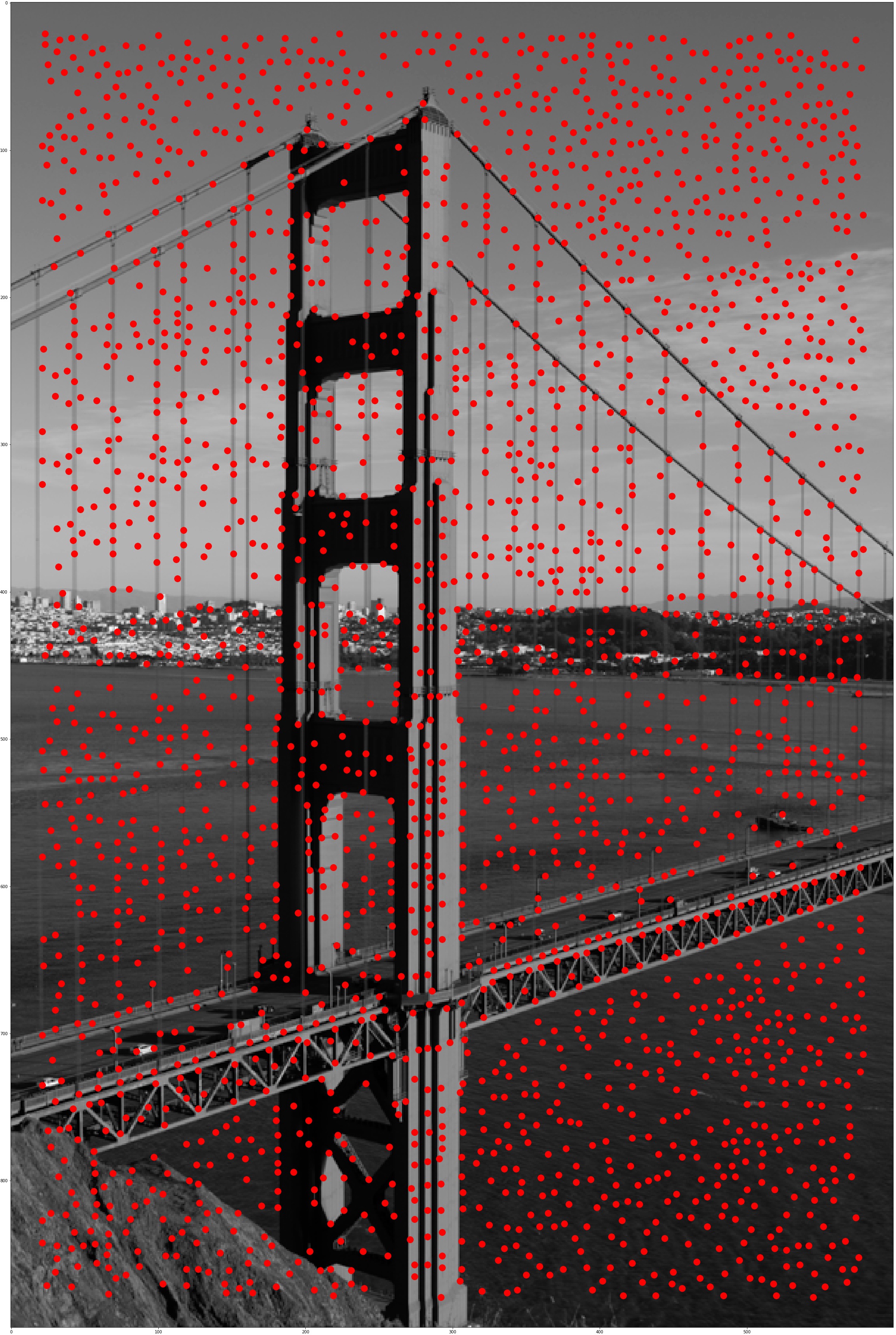
Harris Corner Detector finds corners in an image, which can be potential point of interest in feature matching. I use skimage.feature.corner_harris and skimage.feature.peak_local_max and set the min_distance to 5 to generate a reasonable number of interest points.
Adaptive Non-Maximal Suppression
The paper proposed an algorithm, Adaptive Non-Maximal Suppression (ANMS) to further limit the maximum number of interest points found as well as to make sure the interest points are well distributed over the image. ANMS algorithm selects the points with the largest minimum suppression radius of point. Here I use a threshold of 500 for number of points selected, and the result are shown below:
Corners After ANMS |
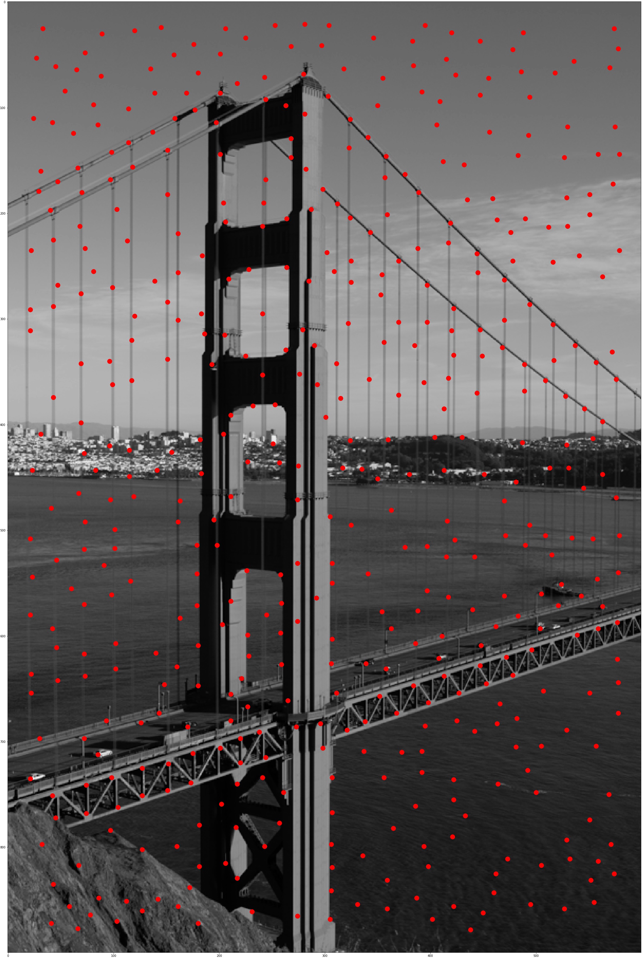
Corners After ANMS |
Feature Descriptor
After obtaining interest points, we now need a feature descriptor to extract the features at the interest points. I extract axis-aligned 40x40 patches and downsampling them to 8x8 to have nice big blurred descriptors that eliminate high frequencies. Then I normalize the patches and output them as 1x64 vectors for each interest point.
Feature Matching
With the feature descriptors we can compare the features at interest points of two images and find good match between them. I use squared distance the metric to determine difference between two sets of points. Then I use 0.6 as the Lowe's threshold on the ratio between the first and the second nearest neighbors. The "good matches" after feature matching and thresholding are shown below:
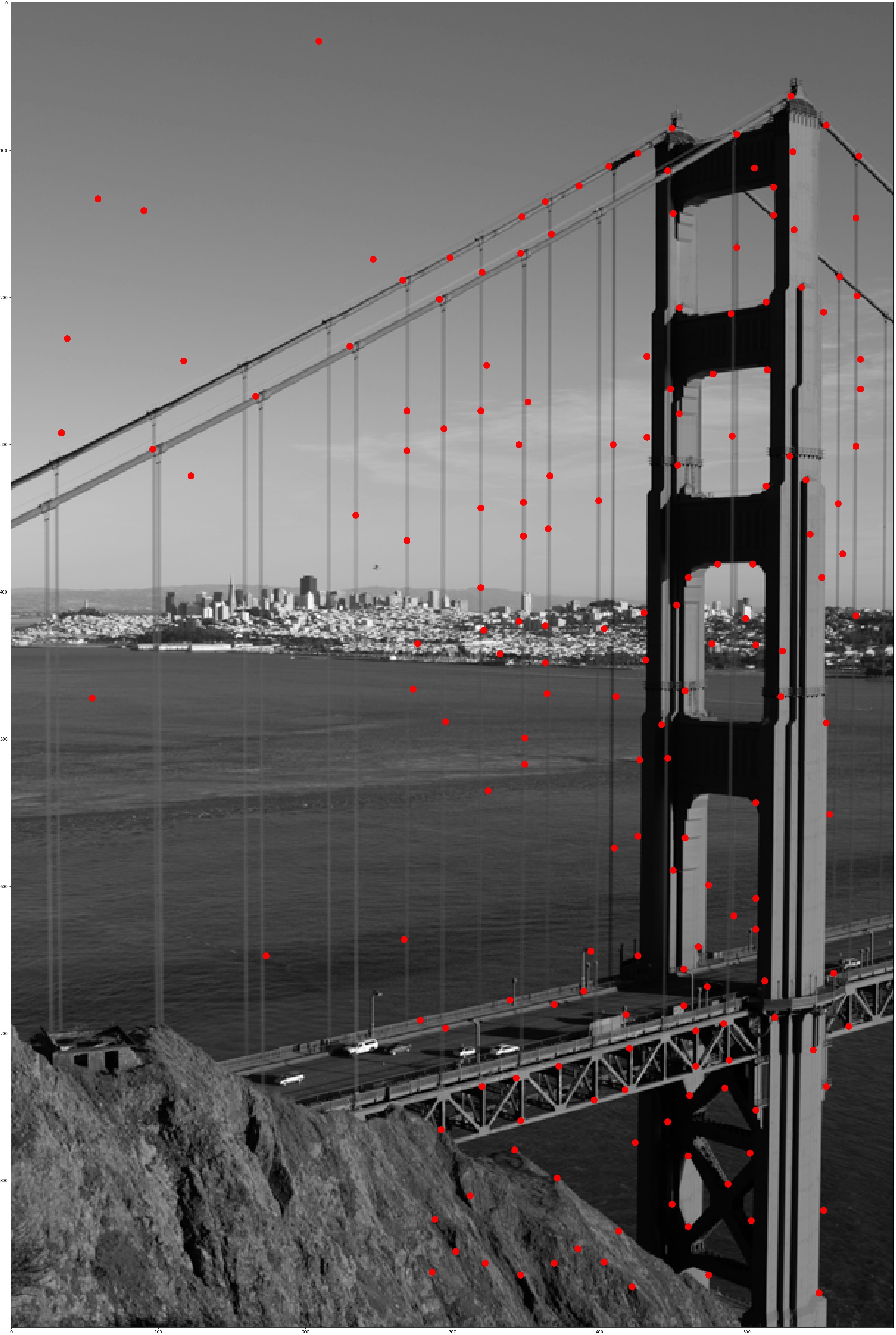
Interest Points After Feature Matching |
Interest Points After Feature Matching |
Random Sample Census (RANSAC)
We can reject outliers using RANSAC to generate a robust homography estimate. Here I randomly choose 4 sets of matching points, compute a homography betweem them, warp all matching points from first image into the homography, compute the SSD between the warped results and real matches in the second images, and threshold on the error to find the inliers. I set my error threshold to be 0.2 and repeat the above process for 300 iterations to find the best homography that produces the most 'real matching pairs'. The 'real matching pairs' after RANSAC are shown below:
Interest Points After RANSAC |
Interest Points After RANSAC |
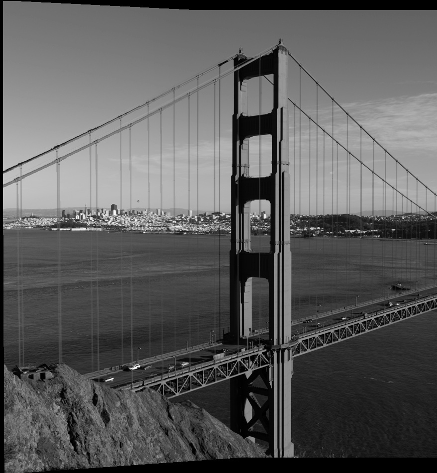
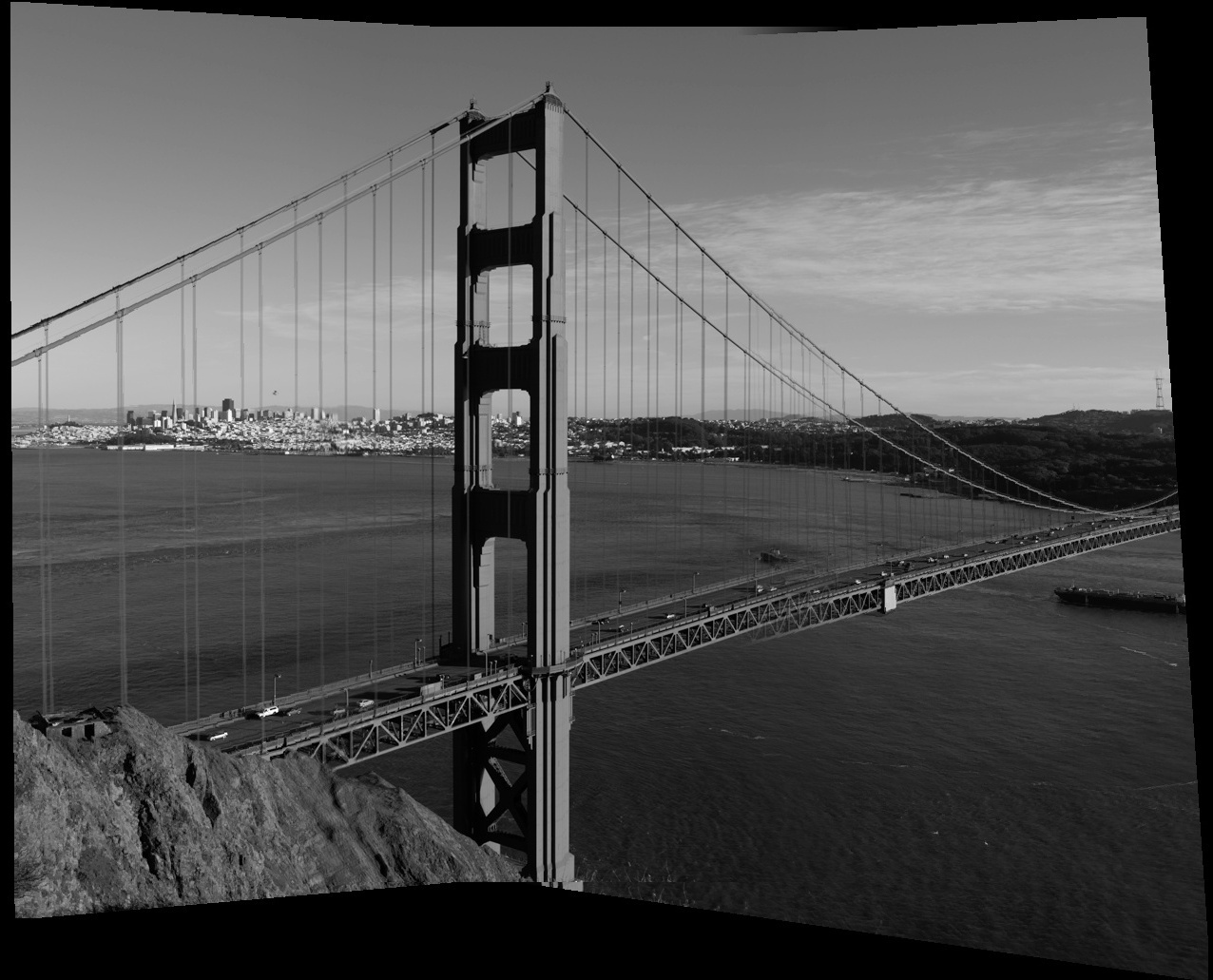
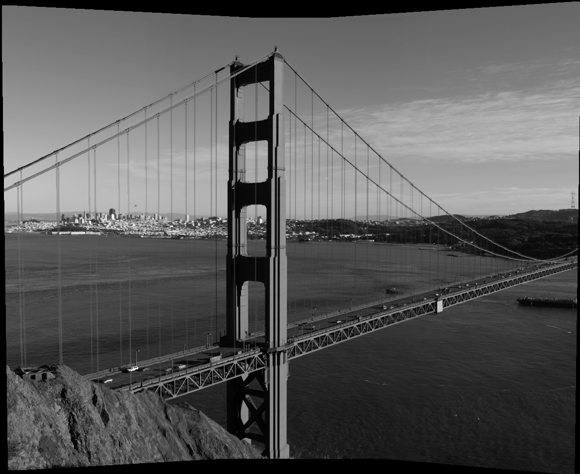
Golden Gate Mosaic after RANSAC |
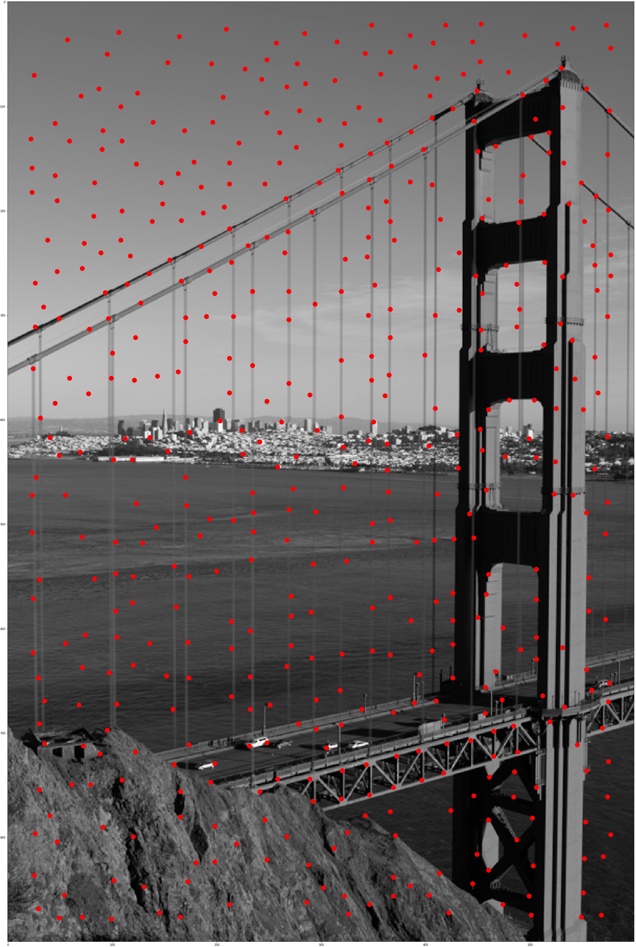
A progress in detecting interest points:
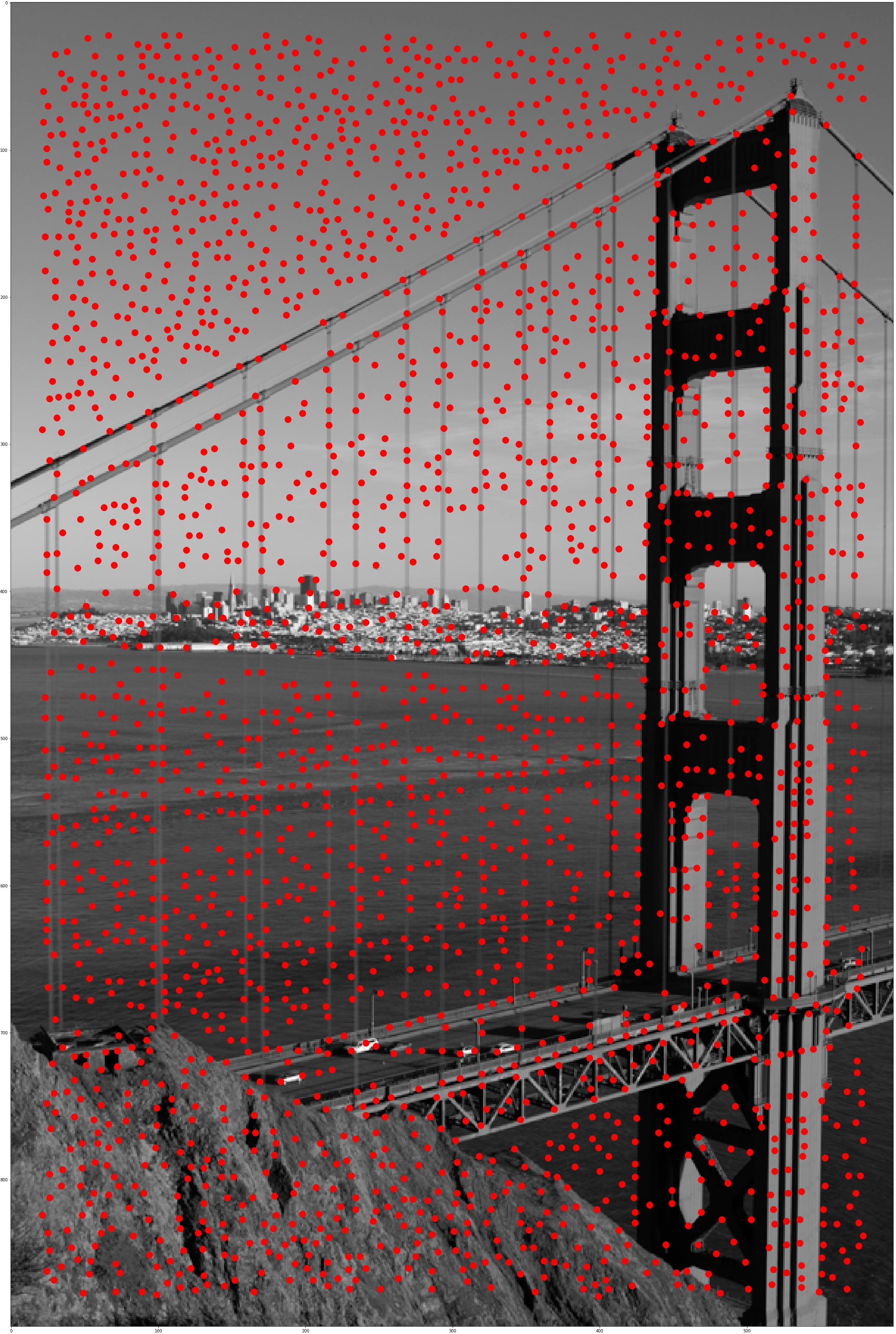
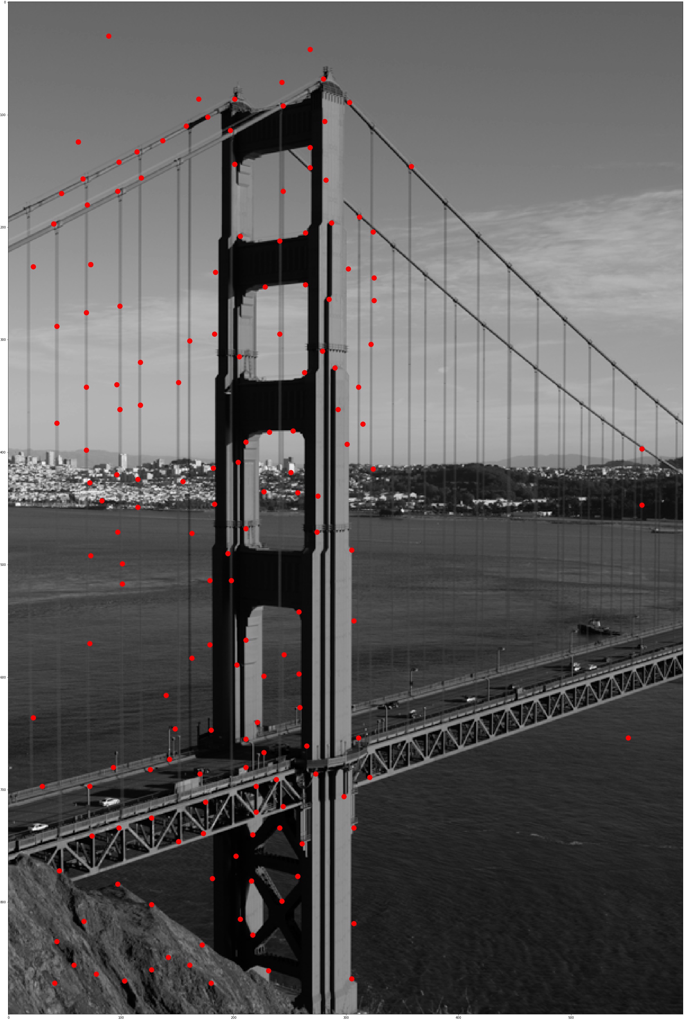
2534 Interest Points After Harris Corner |
500 Interest Points After ANMS |
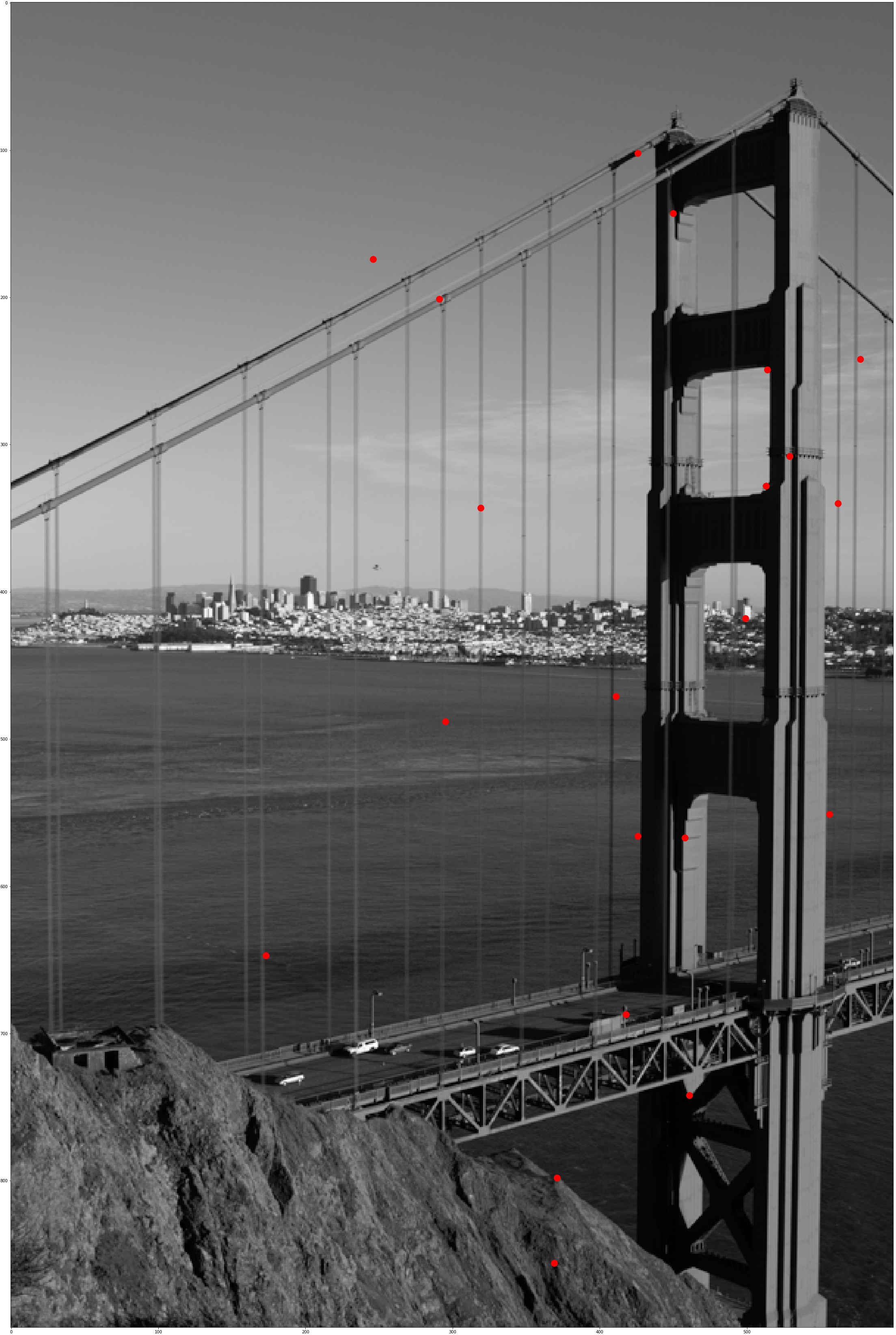
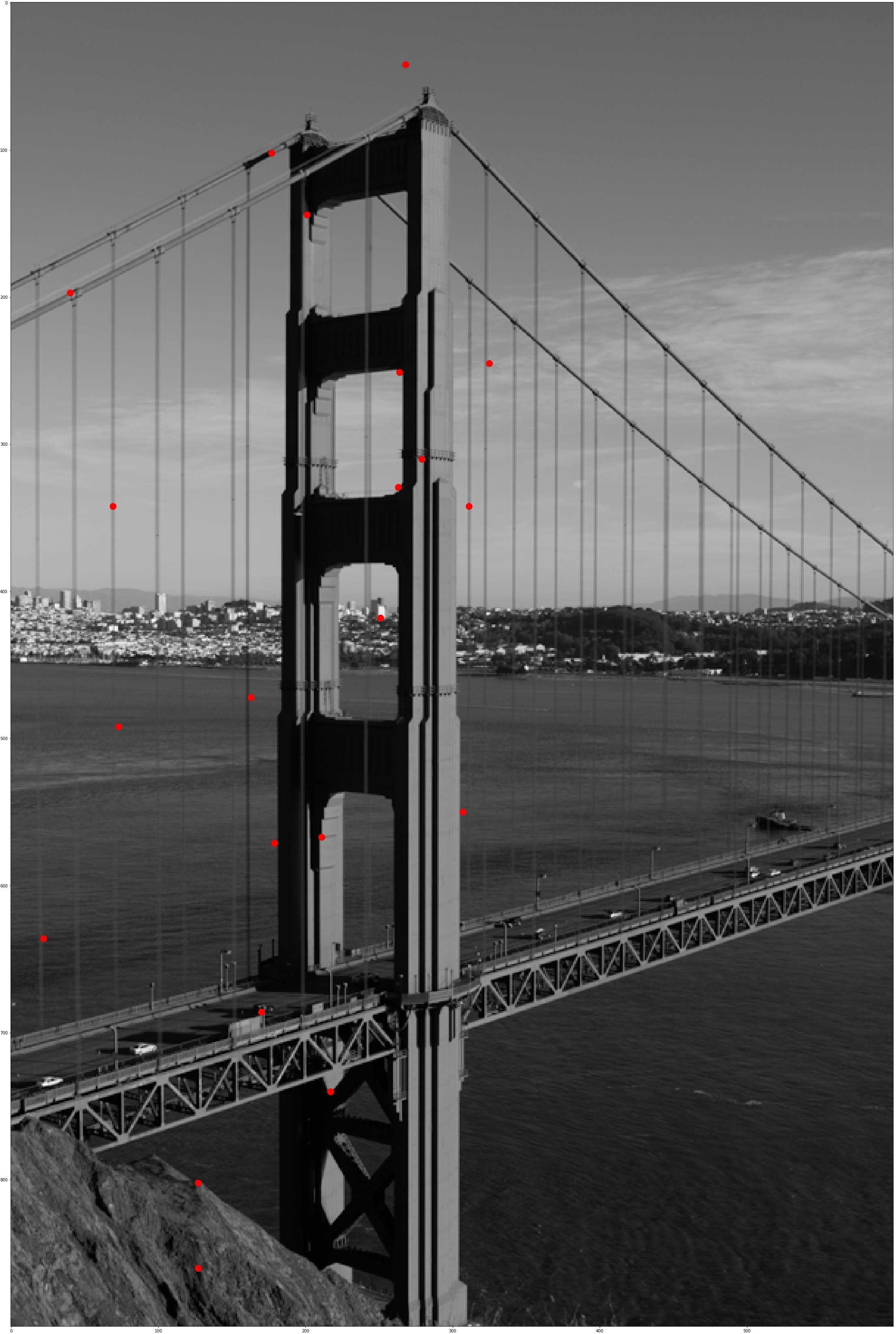
179 Interest Points After Feature Matching |
21 Interest Points After RANSAC |
Result
Here are the comparison between mosaic by manually selected correspondences (on the left) and mosaic by automatic feature matching (on the right). We can see visible difference in the golden gate mosaic pair, as the manually matched one has some clear error in matching the center and right image, which might result from minor errors in declaring correspondences. The rest of mosaics doesn't show a visible difference, only that the manually matches ones are sometimes blurry while the auto-matched ones always has a great resolution.
What I Learned
The coolest thing I learned is making an automatic feature detector and feature matcher. Constructing a feature extracter is almost like teaching the computer to view images like human do, to see certain aspects from the scene, and even to understand the scene's composition.