[Auto]Stitching Photo Mosaics

A CS 194-26 project 5 by Xiangtian Li, cs194-26-agr

Part 1: Image Warping and Mosaicing

Recover Homographies

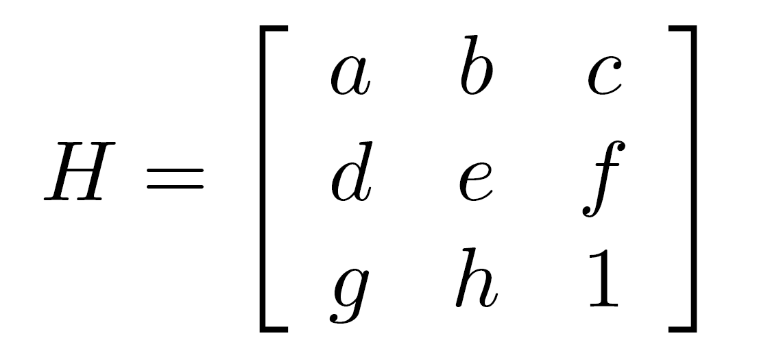
The 3*3 homography matrix has the following form

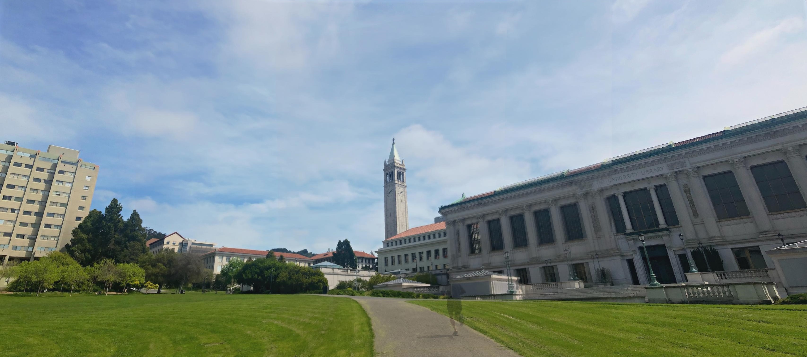
Given n pairs of points of the first image and the second image, we want to find H to minimized the following cost

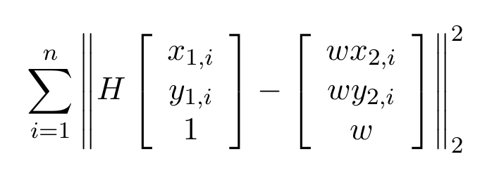
Then we can use least square method to recover H

Image Warping and Rectification

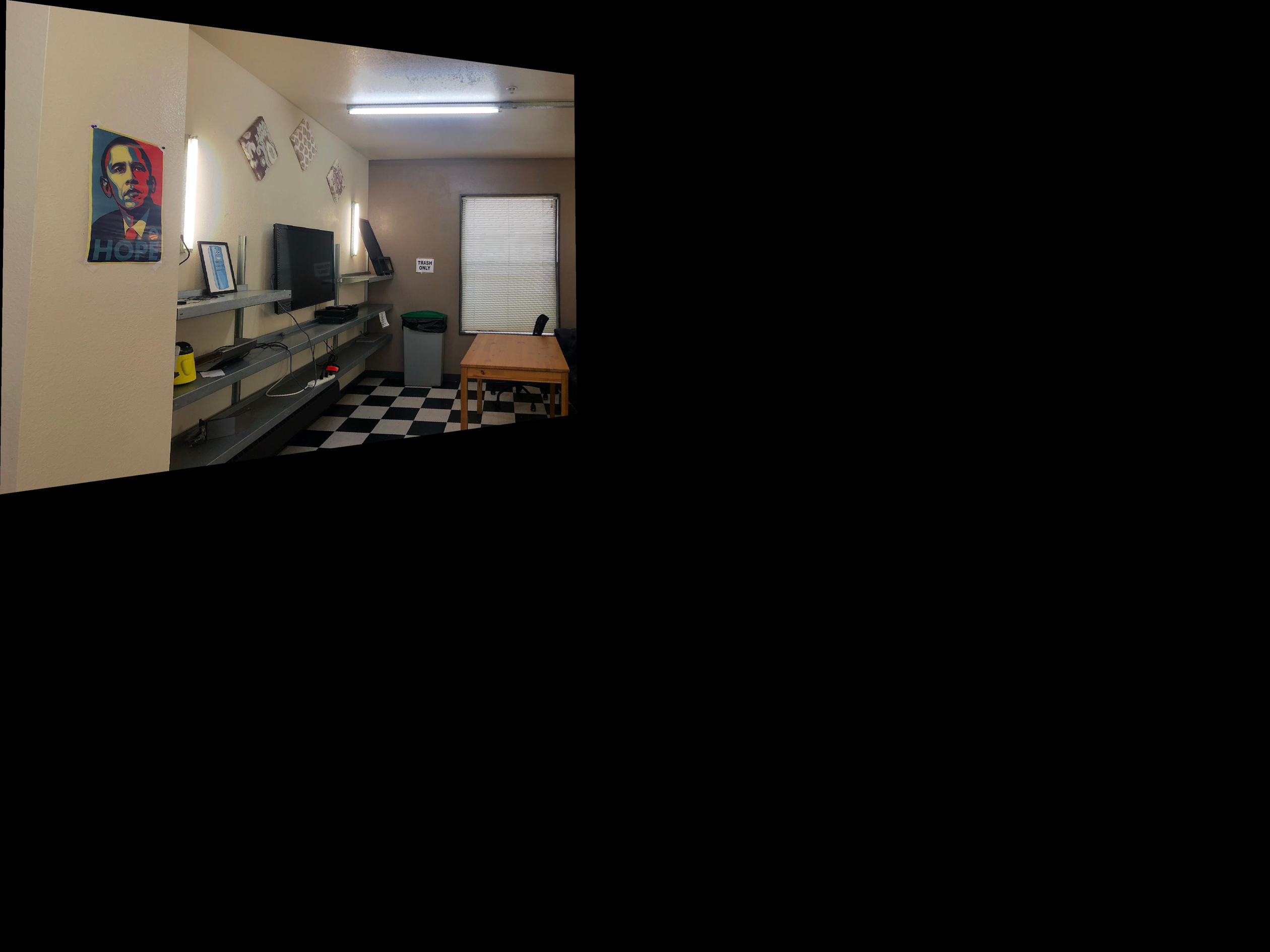
We use the inverse matrix to implement warping. By multiplying the coordinates into the original image, we can get a new warping image.

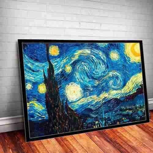
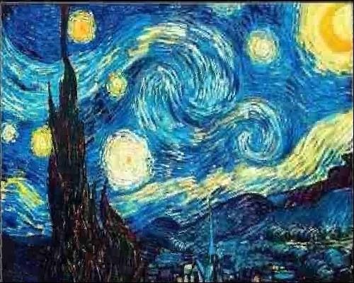
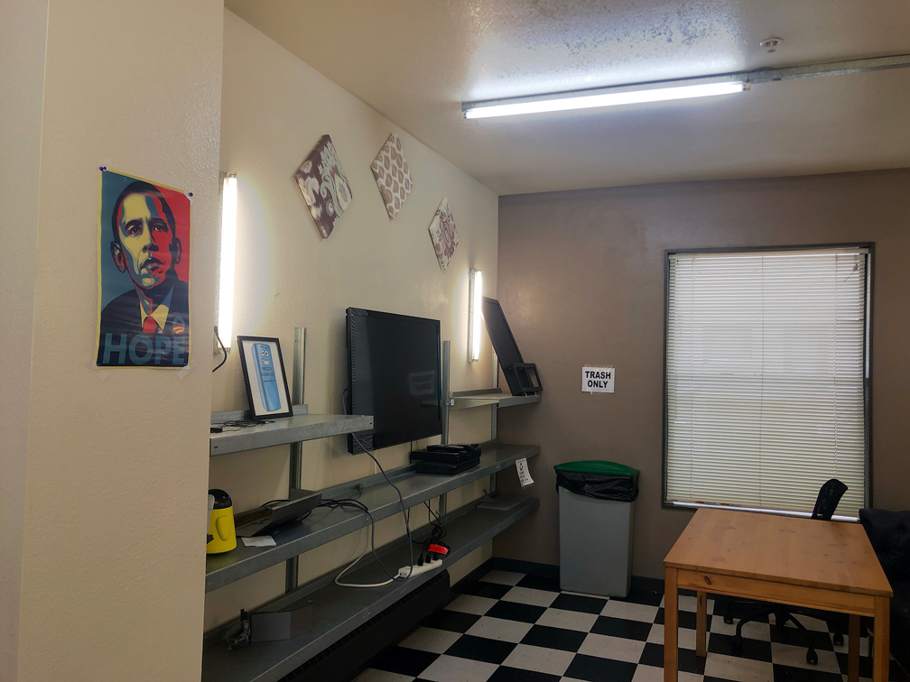
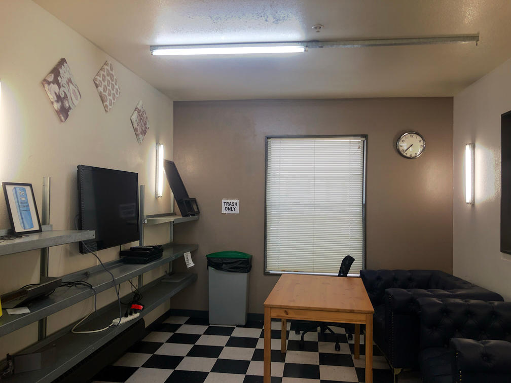
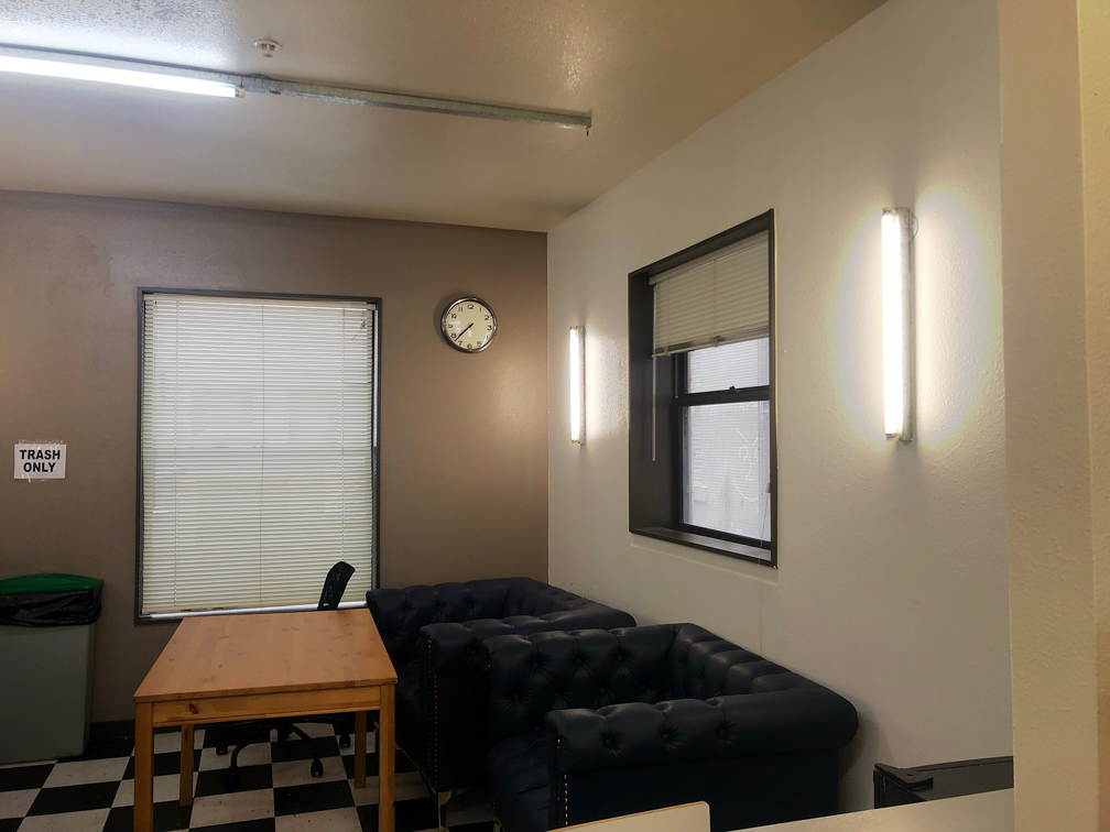
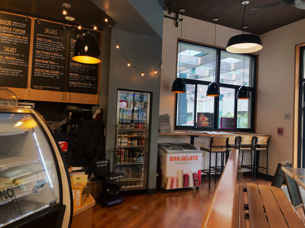
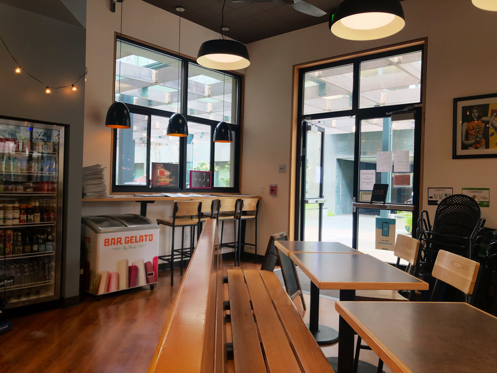
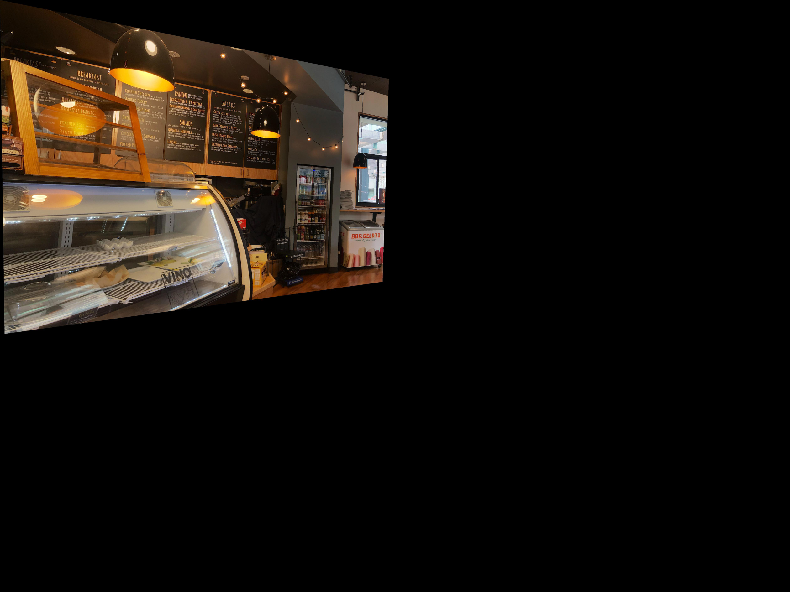
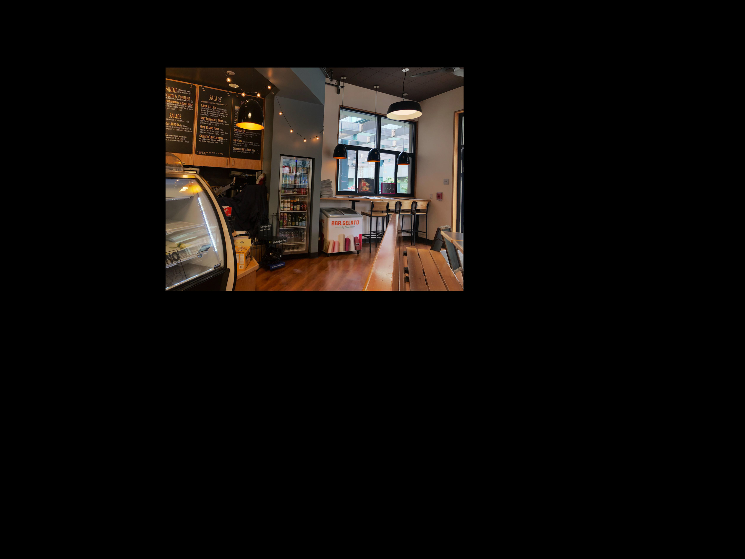
As for image rectification, we simply select 4 points of the object corners in the original image and choose 4 corners in the output image to be rectangle. Below are some example images.

Mosaics

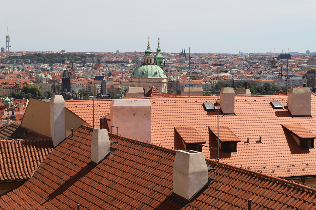
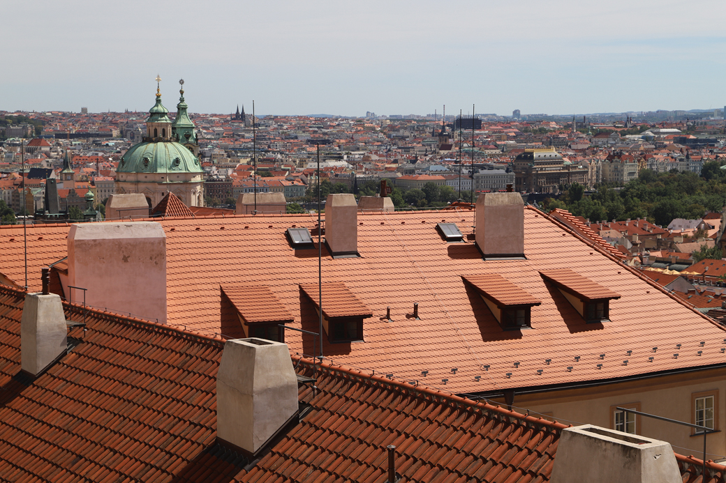
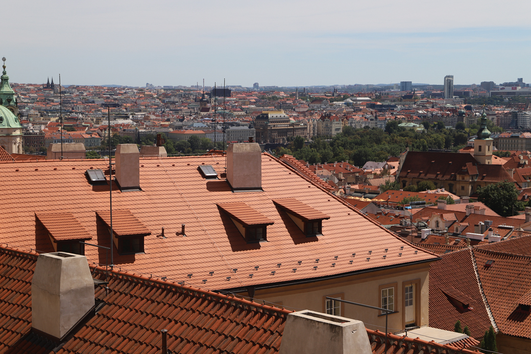
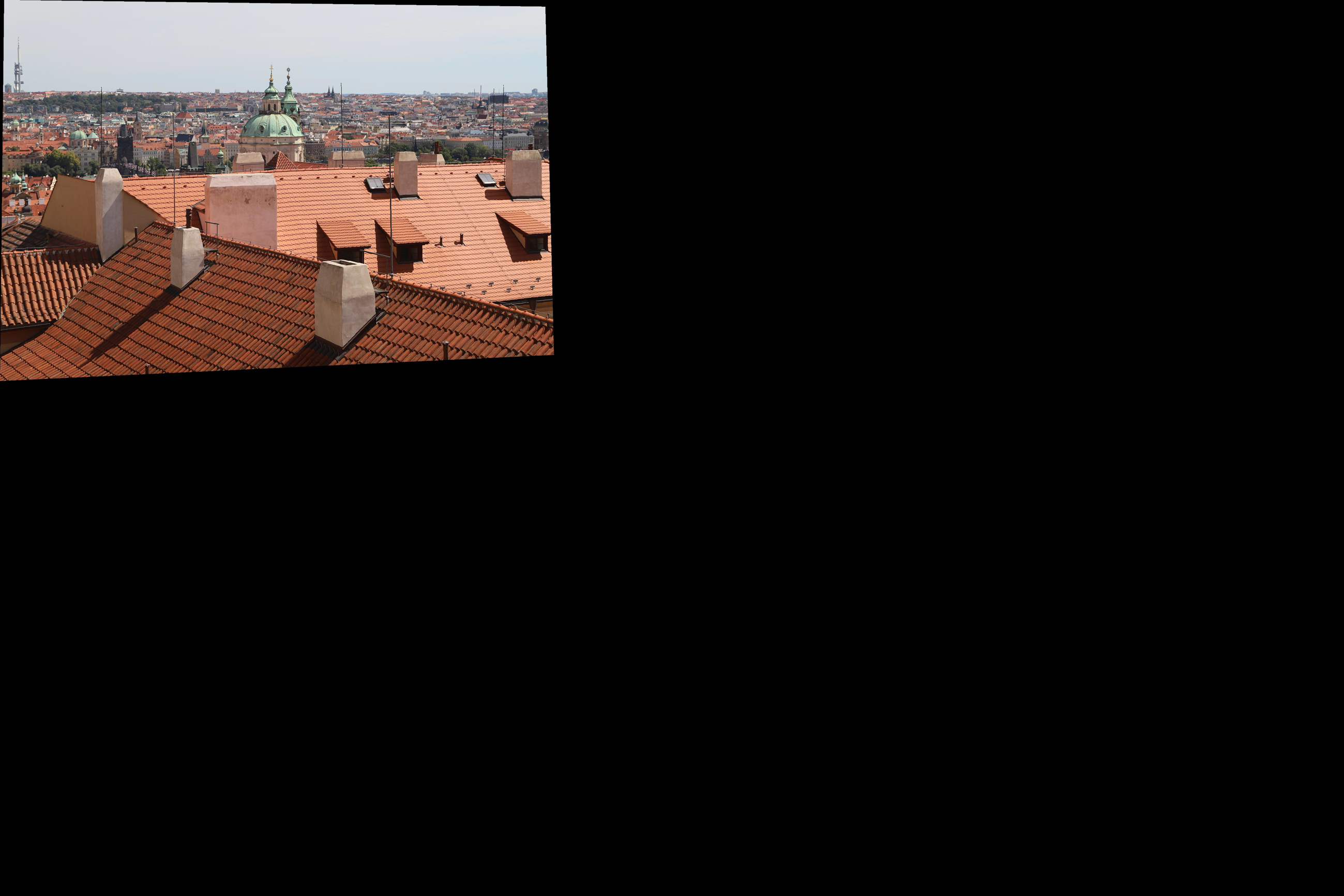
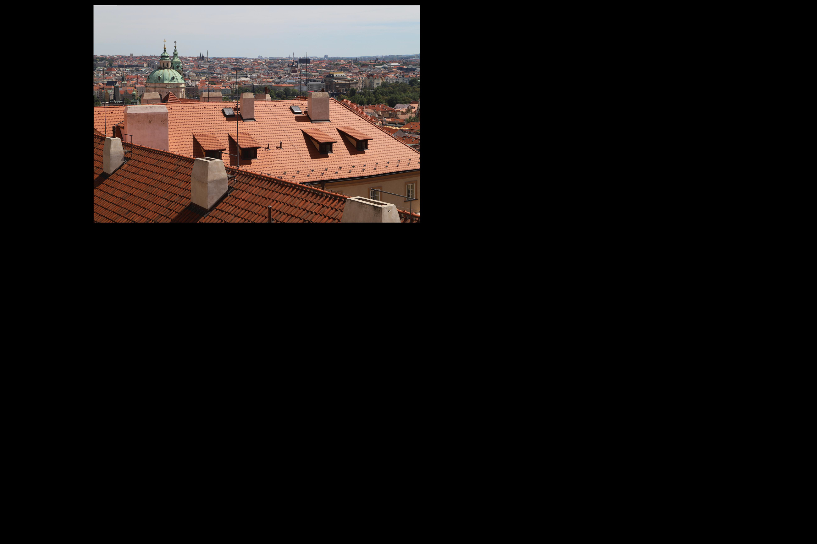
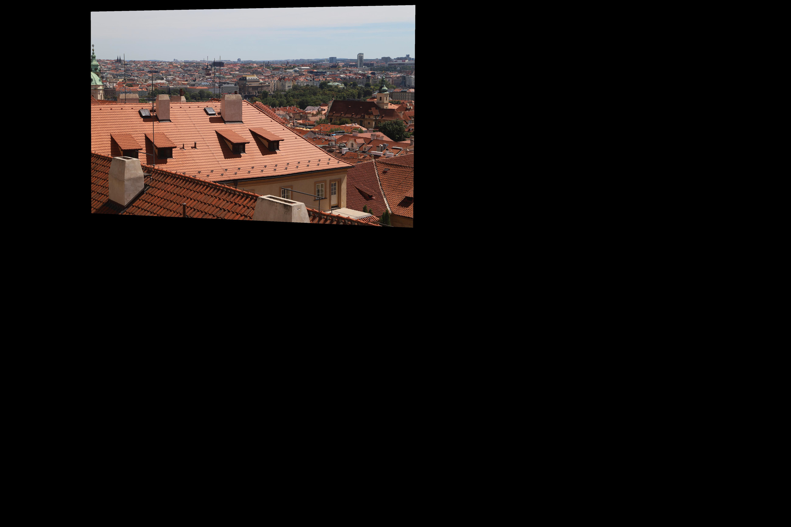
Below are the results

Part2: Automatic Stitching

In this part, we simply implement a simplified version of Multi-Image Matching using Multi-Scale Oriented Patches to achieve automatic stitching.

Harris Corners

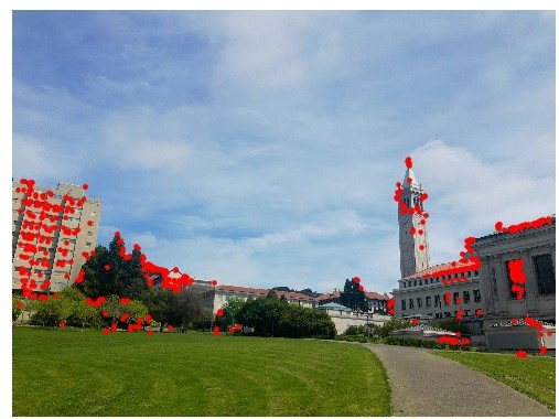
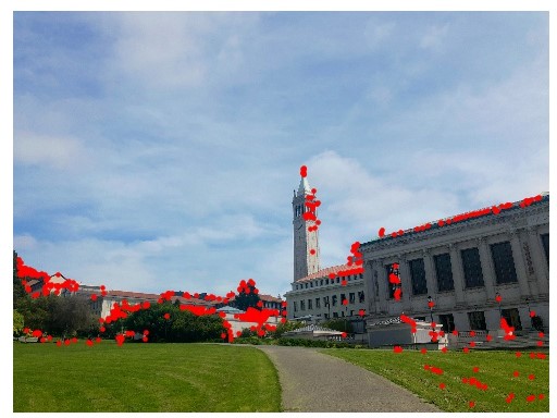
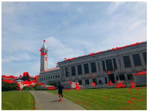
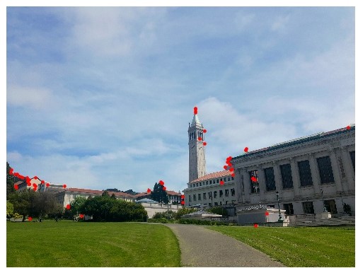
In this part, we use the corner_harris and corner_peaks functions of skimage.feature. We found that corner_peaks can result in much less points than peak_local_max does. Below I show three of the examples.

Adaptive Non-Maximal Suppression

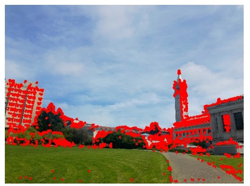
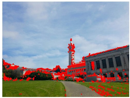
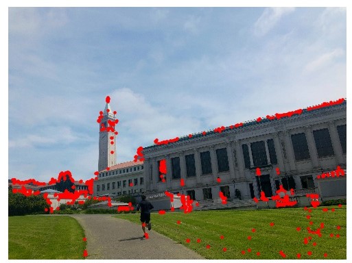
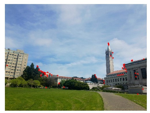
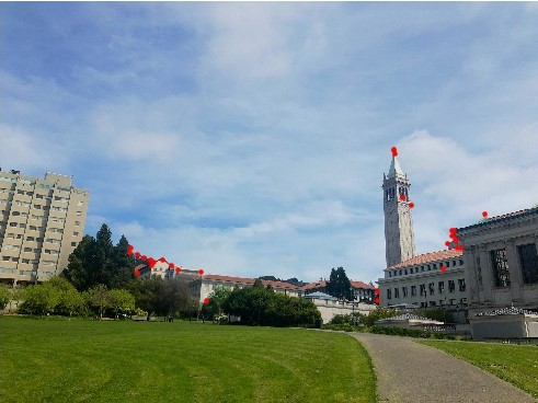
The algorithm presented in the paper, Adaptive Non-Maximal Suppression(ANMS), can reduce the number of points by selecting the points with the largest $r_i$, where $r_i$ is the minimum suppression radius of $x_i$:

$$r_i = \min_{j} | x_i - x_j |, \text{s.t. }f(x_i) < c_{\text{robust}} f(x_j), x_j \in \mathcal{I}$$

In experiment, we set $c_{robust}=0.9$ and always select the top 500 ranked points. The corners left are shown below.

Feature Descriptor Extraction

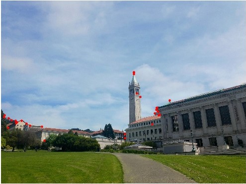
We can descript the feature of points by extracting a $40\times 40$ patch centered at each point and then downsampling it to $8\times 8$. Then we can do bias/gain normalization on the new patch. This can be done by subtracting the mean an dividing by the standard deviation. Then we vectorize the feature descriptors into shape $1\times 64$.

Feature Matching

In this part we find the consistent points in two images. We compute the distance between the feature descriptors of points in the two images. We then sort the distance and use low ratio test: if 1-NN/2-NN is less than some threshold(in the experiment we set it to 0.6), we will consider the pair to be a match. Below we illustrate two matches.

RANSAC

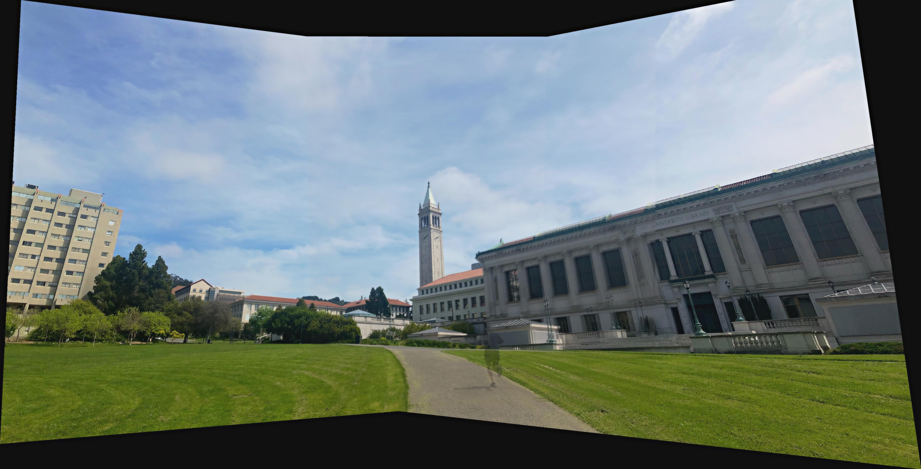
There are some outliers remained in the matches. We can use RANSAC to remove them. First, we randomly choose 4 matches and compute the homography H. Then we warp all points in the first images into the second images and compute the distance between them. We define the points as inliers if their distances are less than a threshold(we set it to 1 in experiment). Iteratively do this for several times and always keep the largest set of inliers and let them to be our best matches.

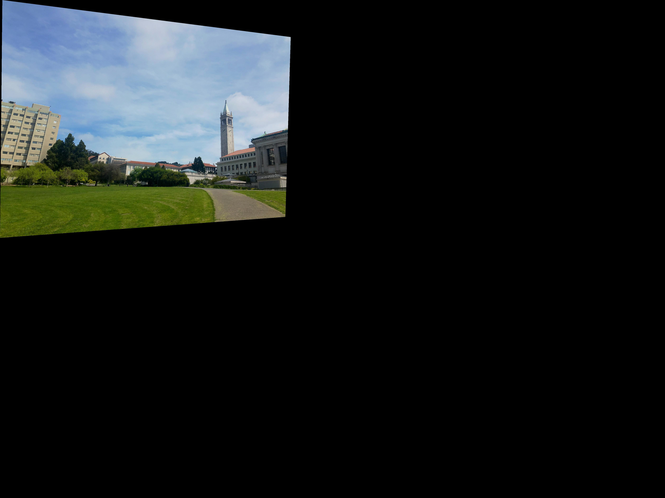
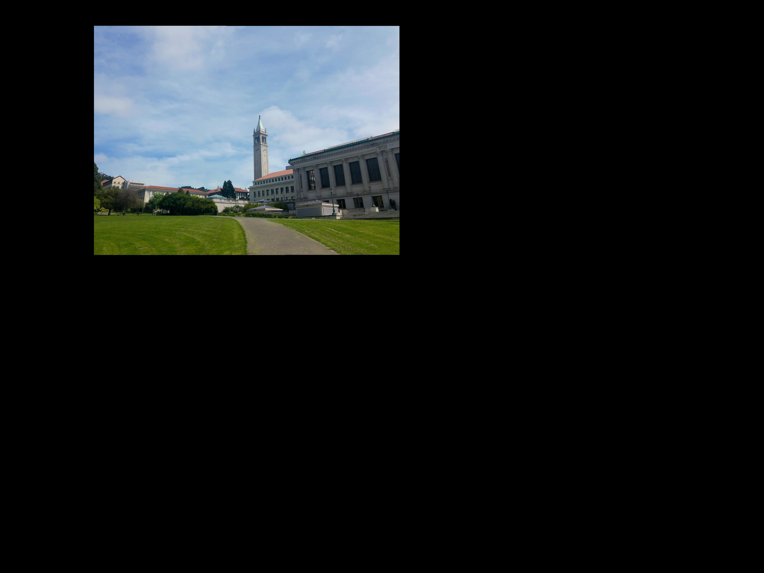
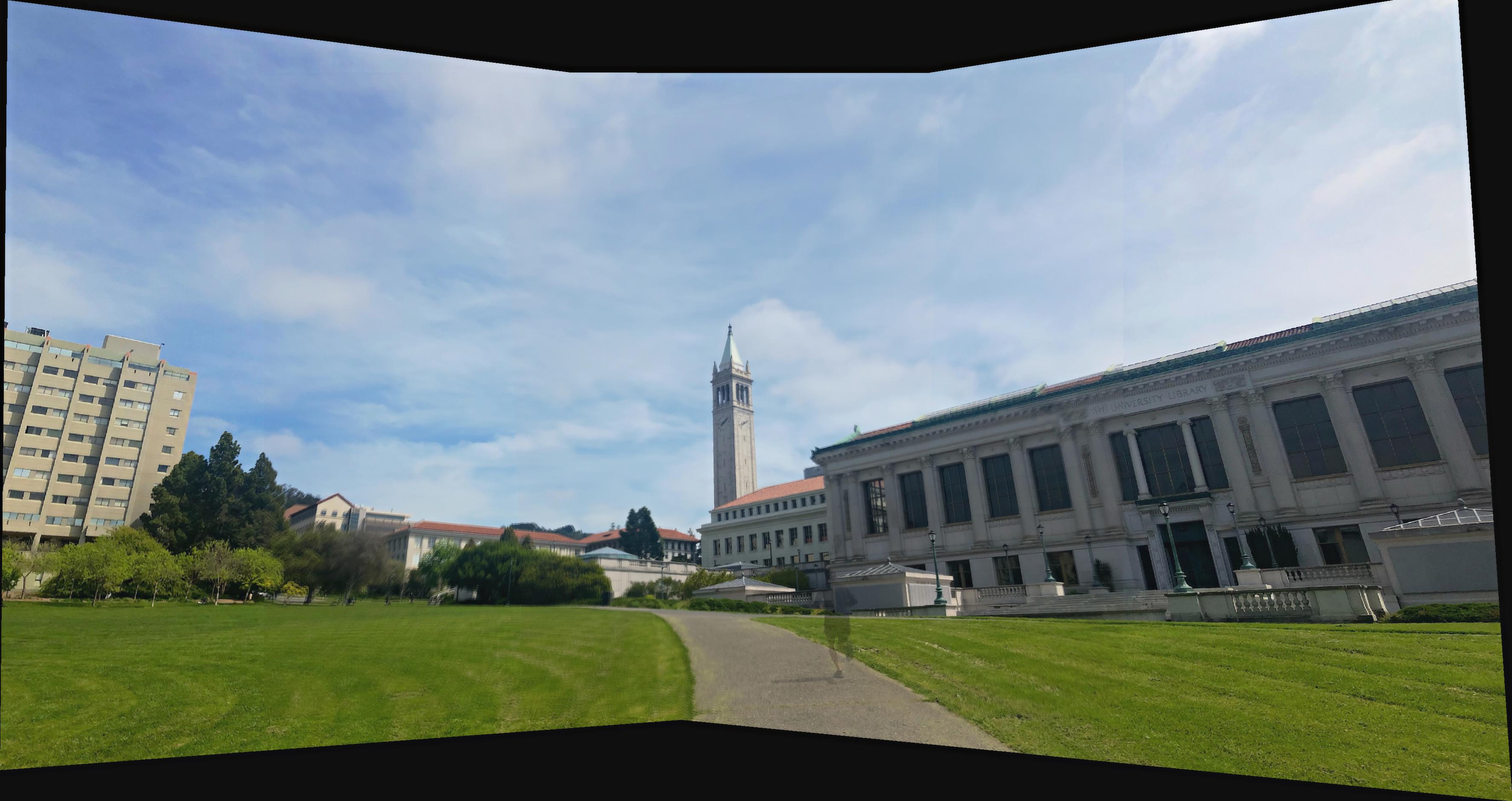
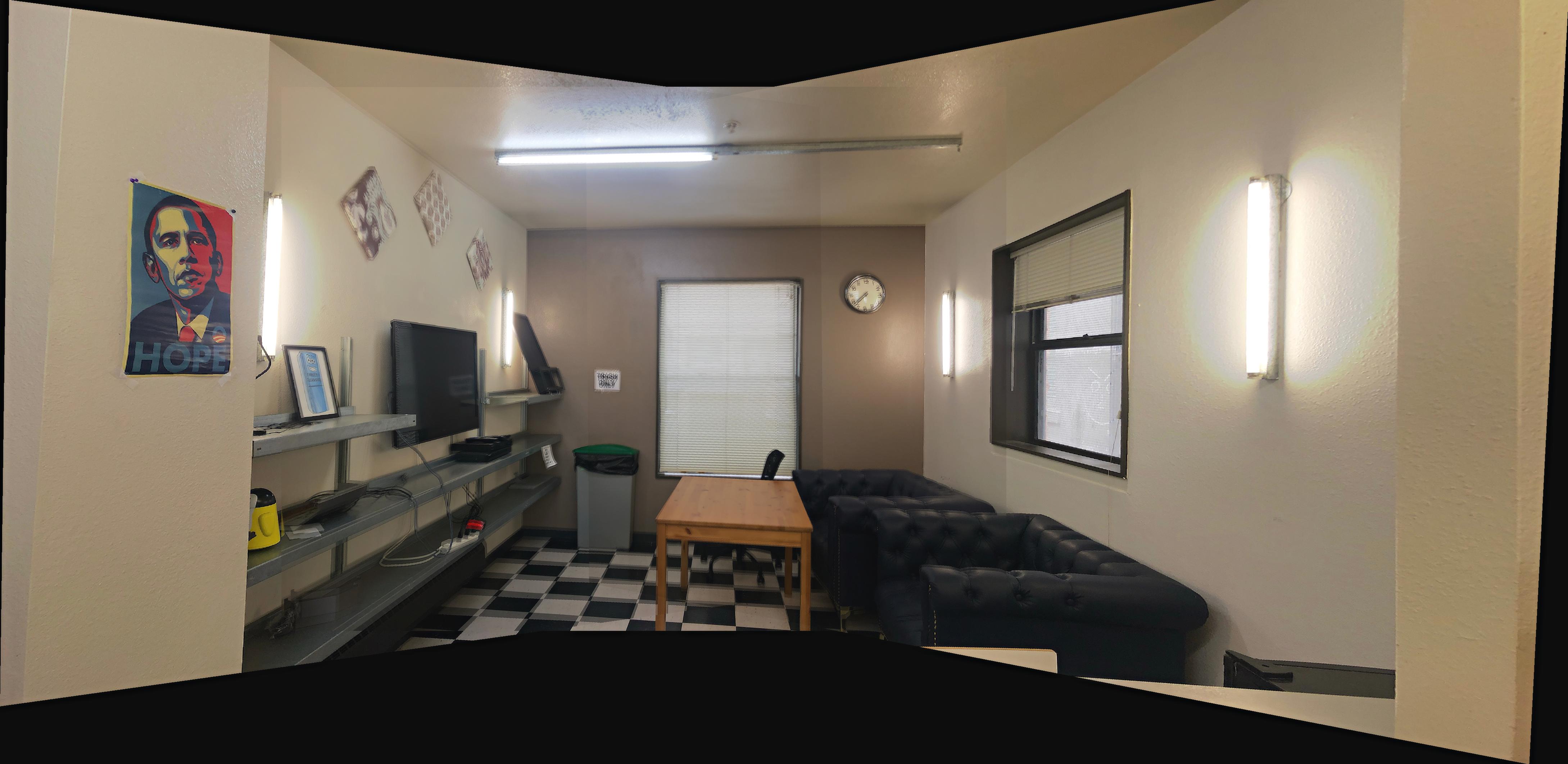
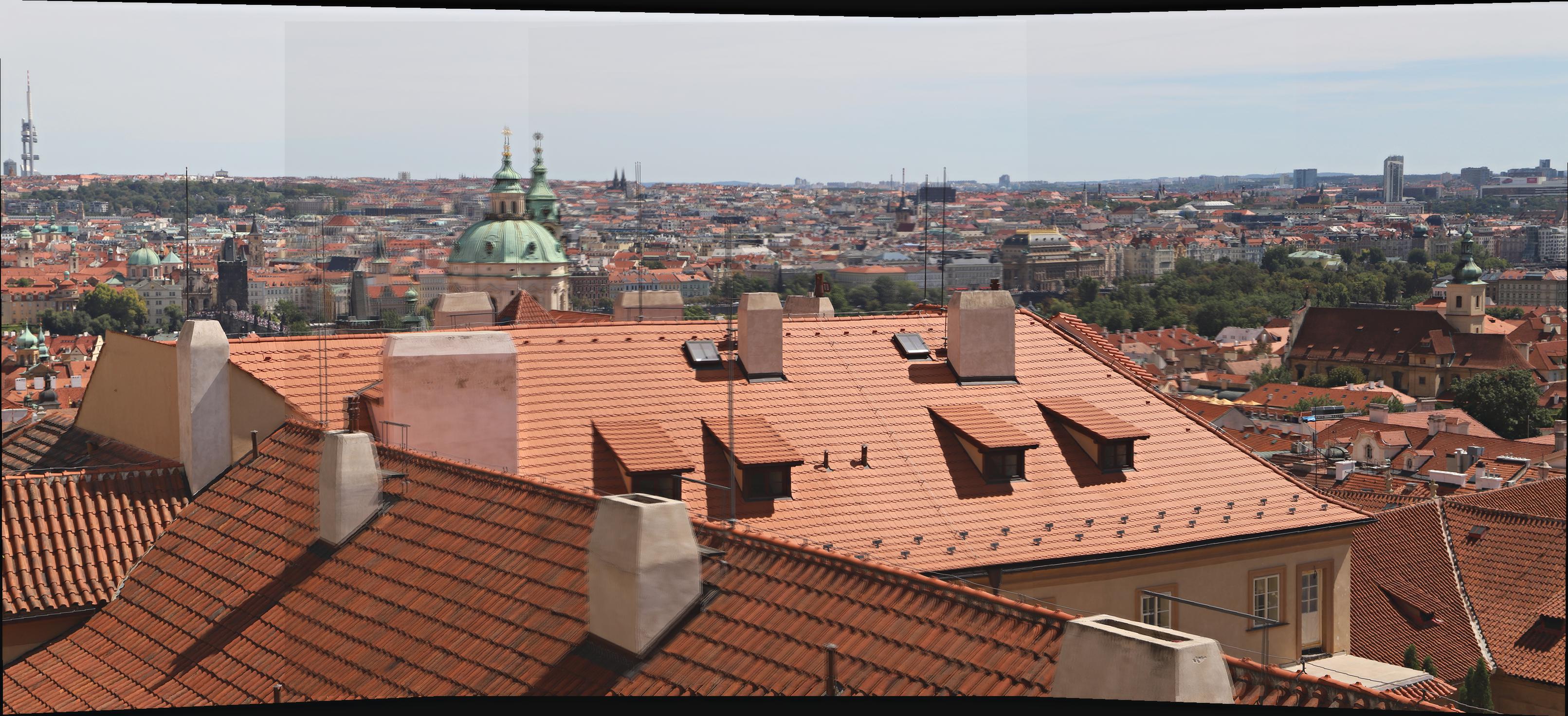
Below we show some matches left after RANSAC. Having gained the matches, we can use the technics in Part1 to warp and blend the images into a panorama.

Results

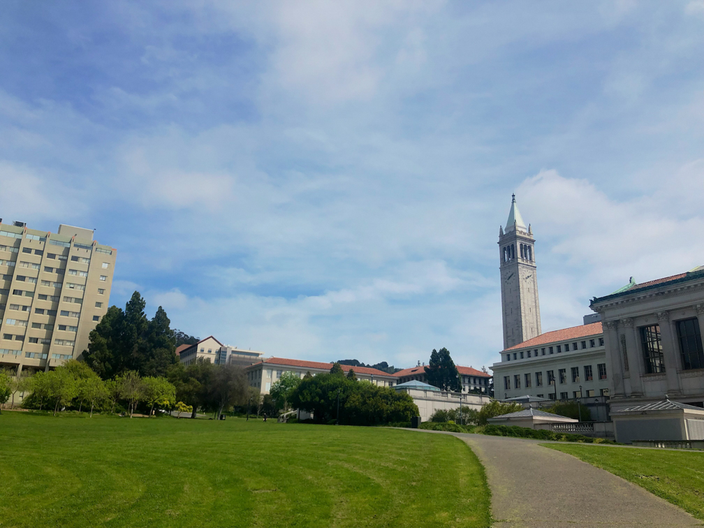
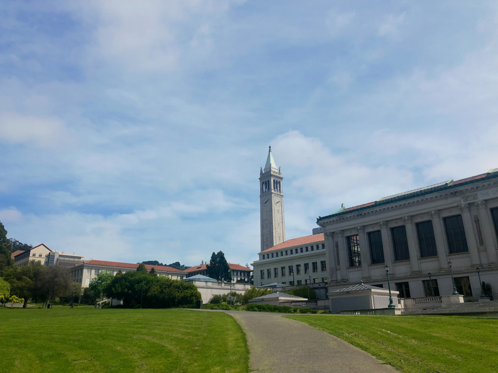
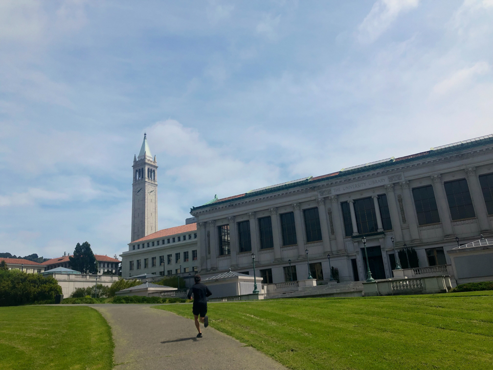
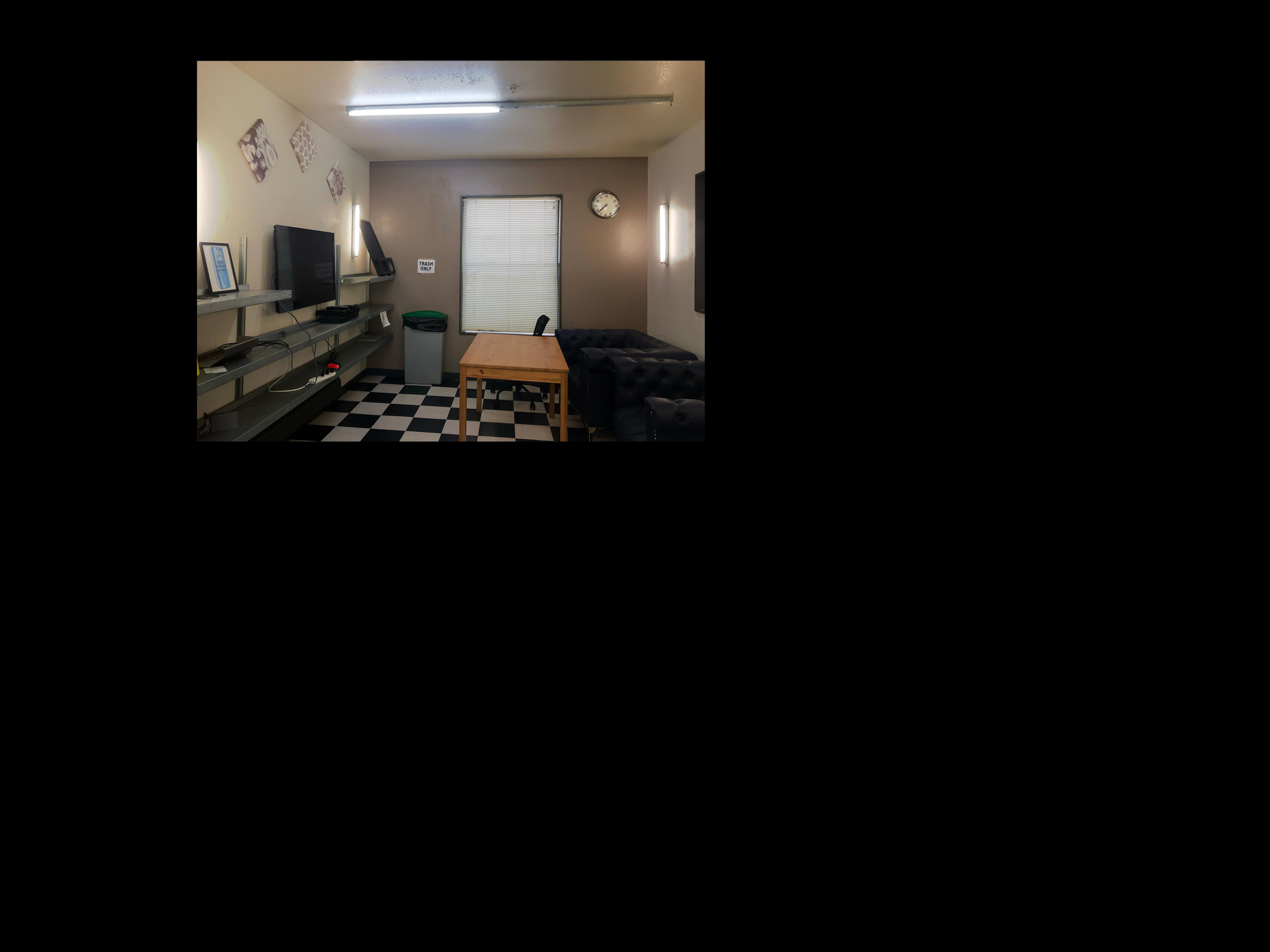
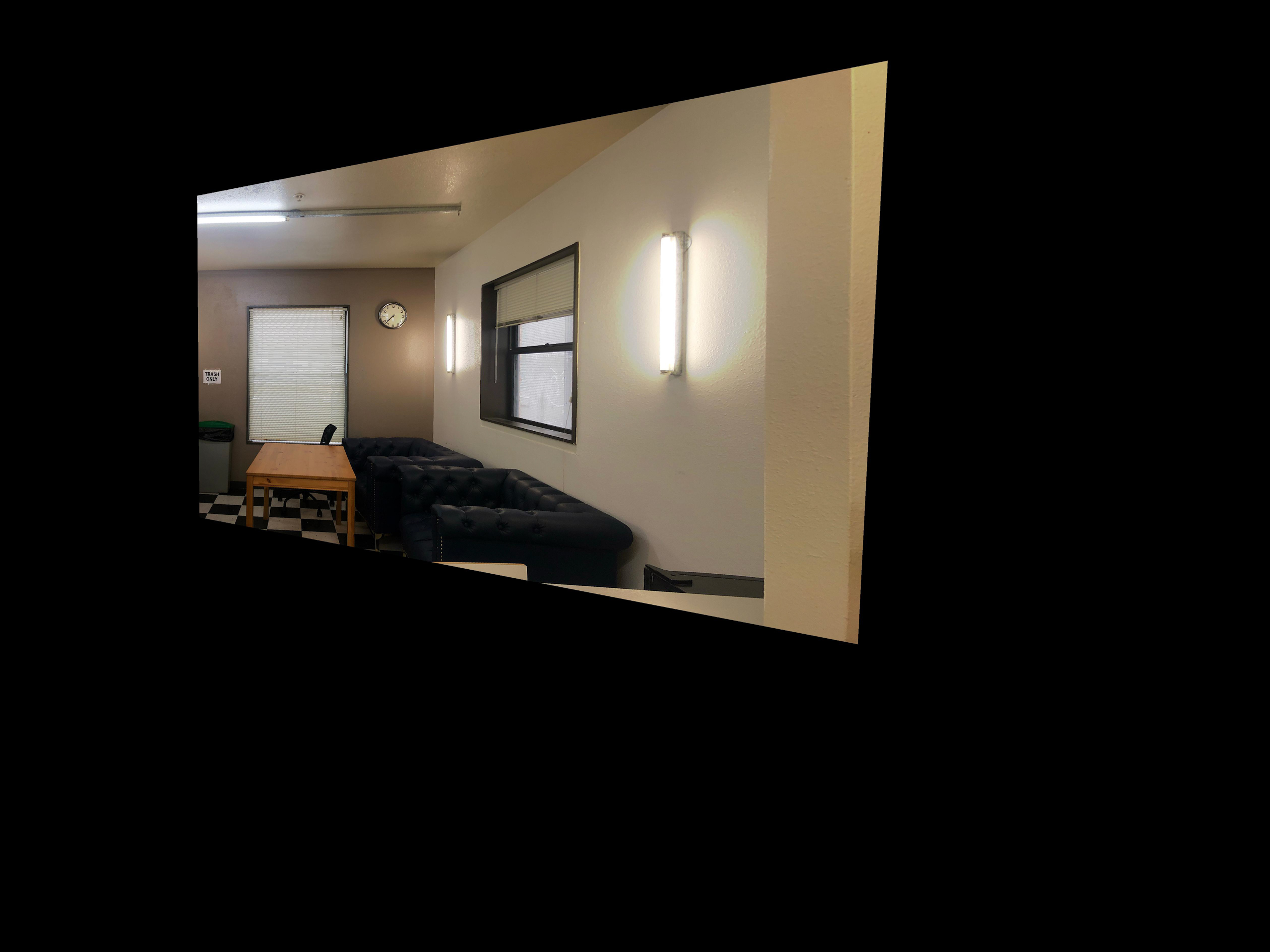
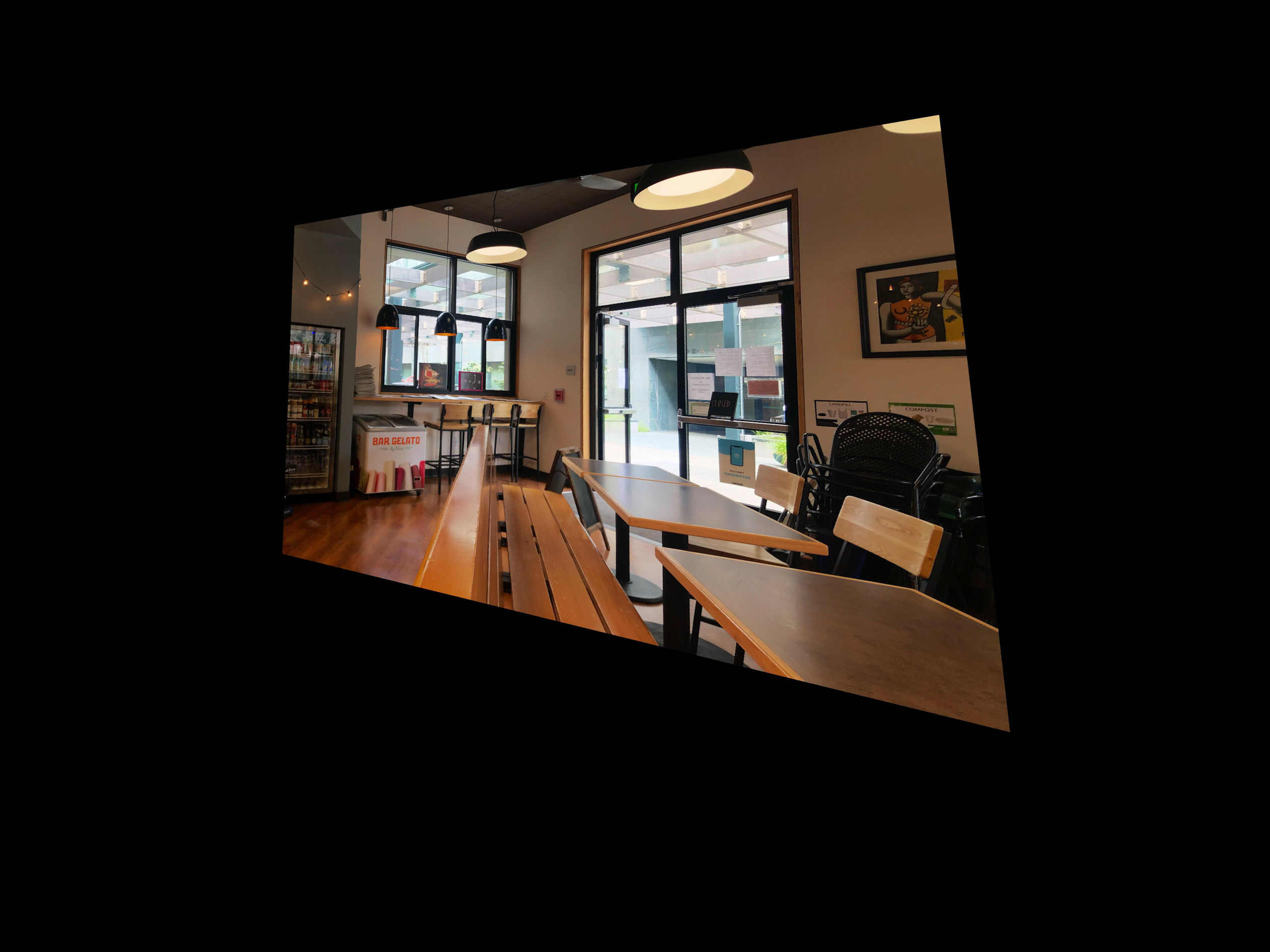
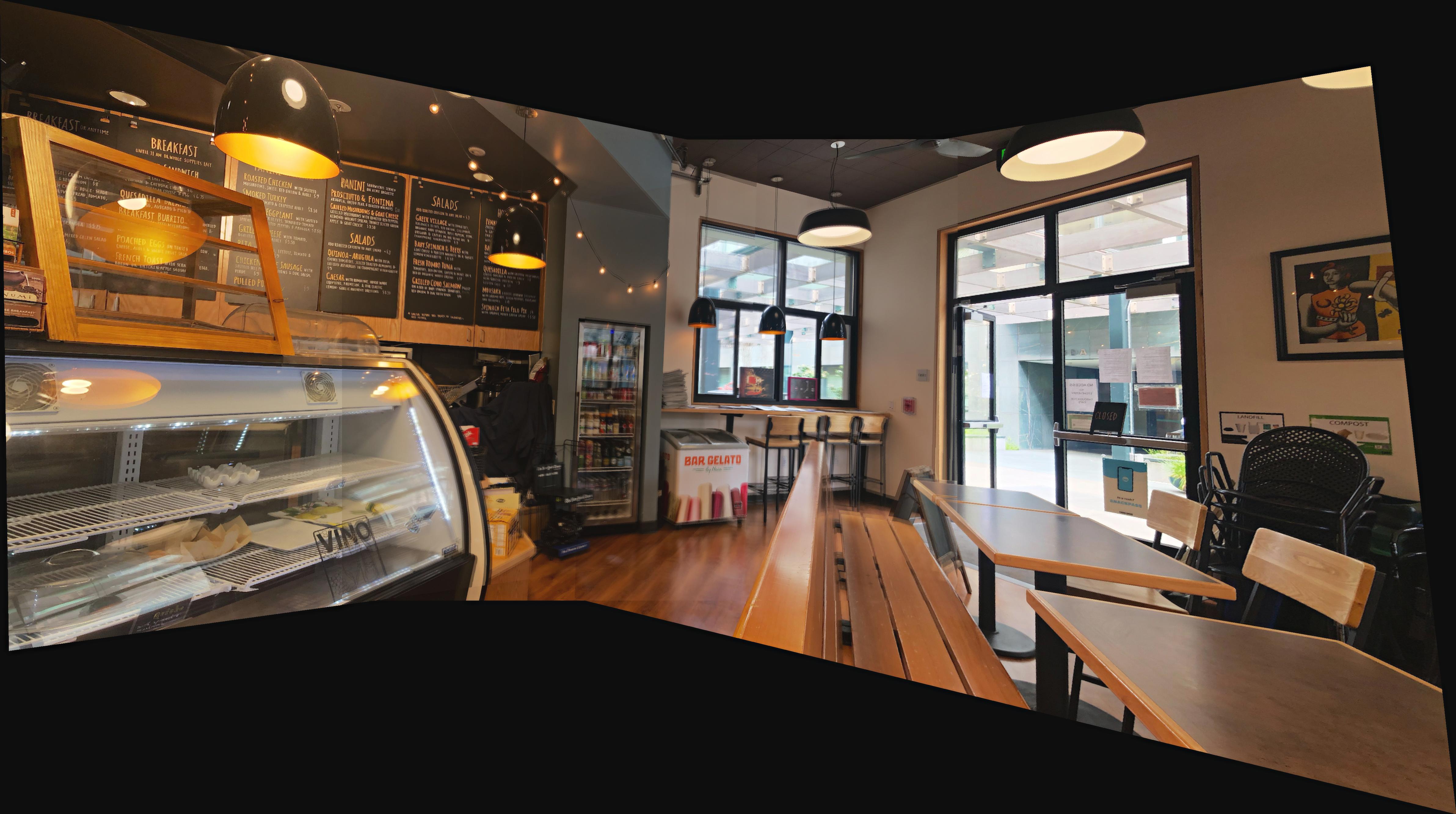
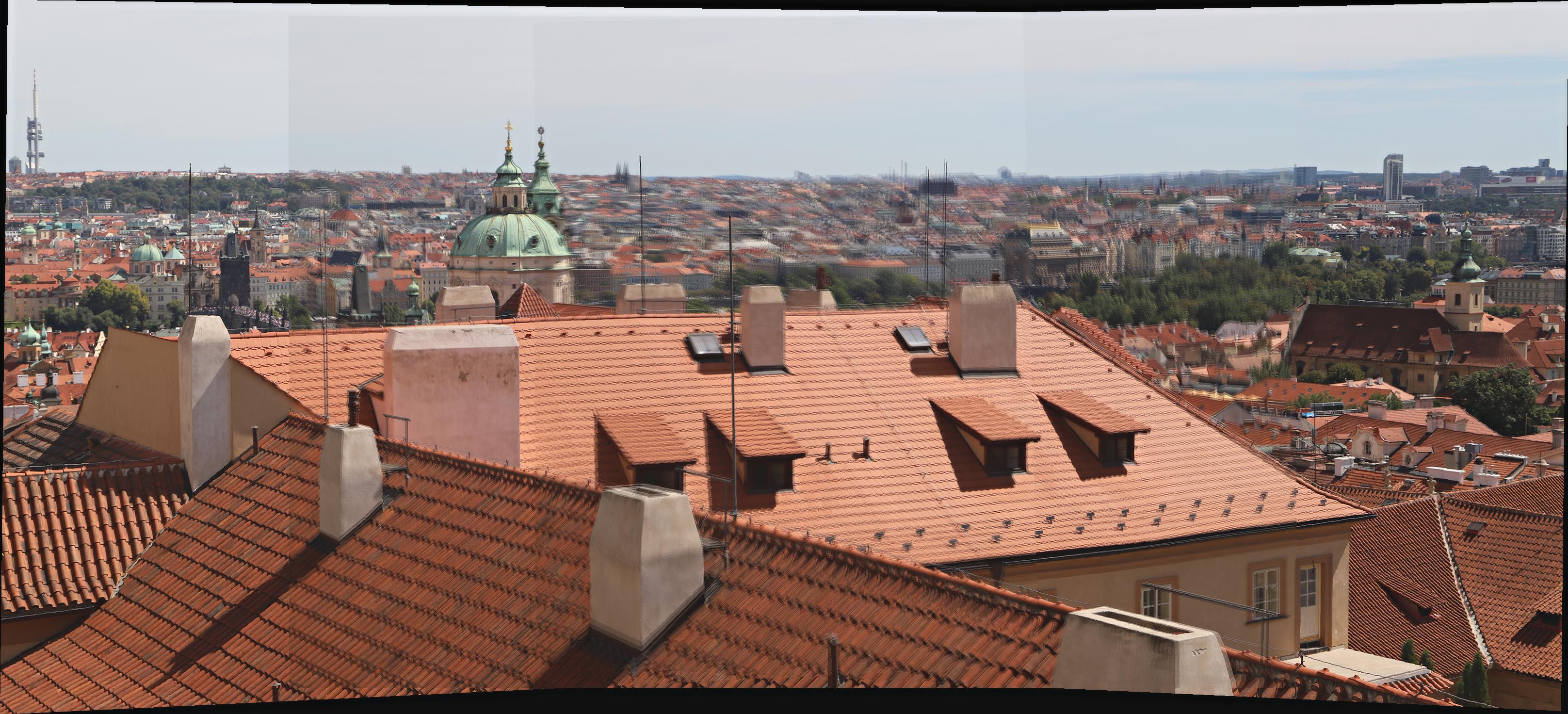
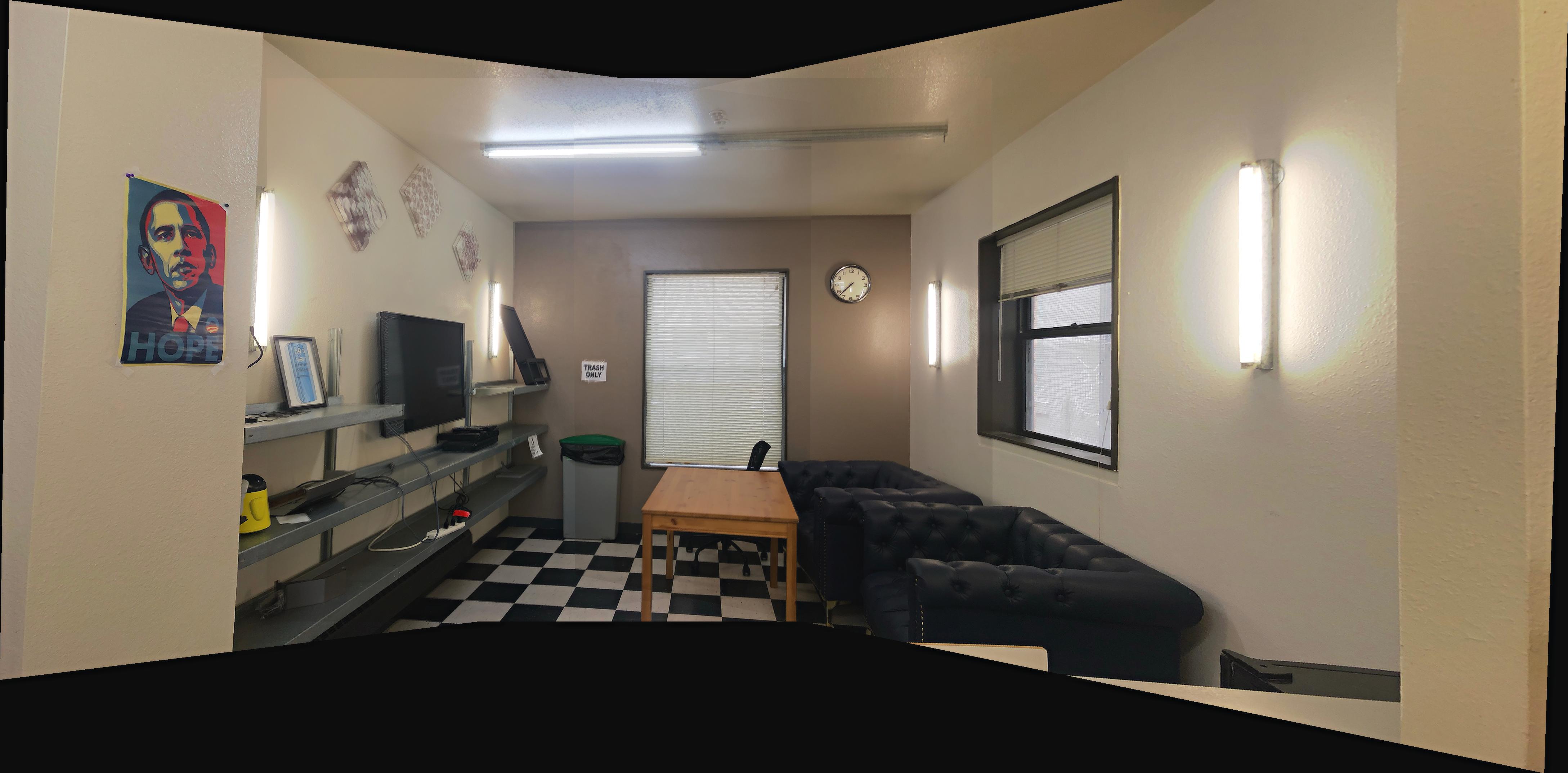
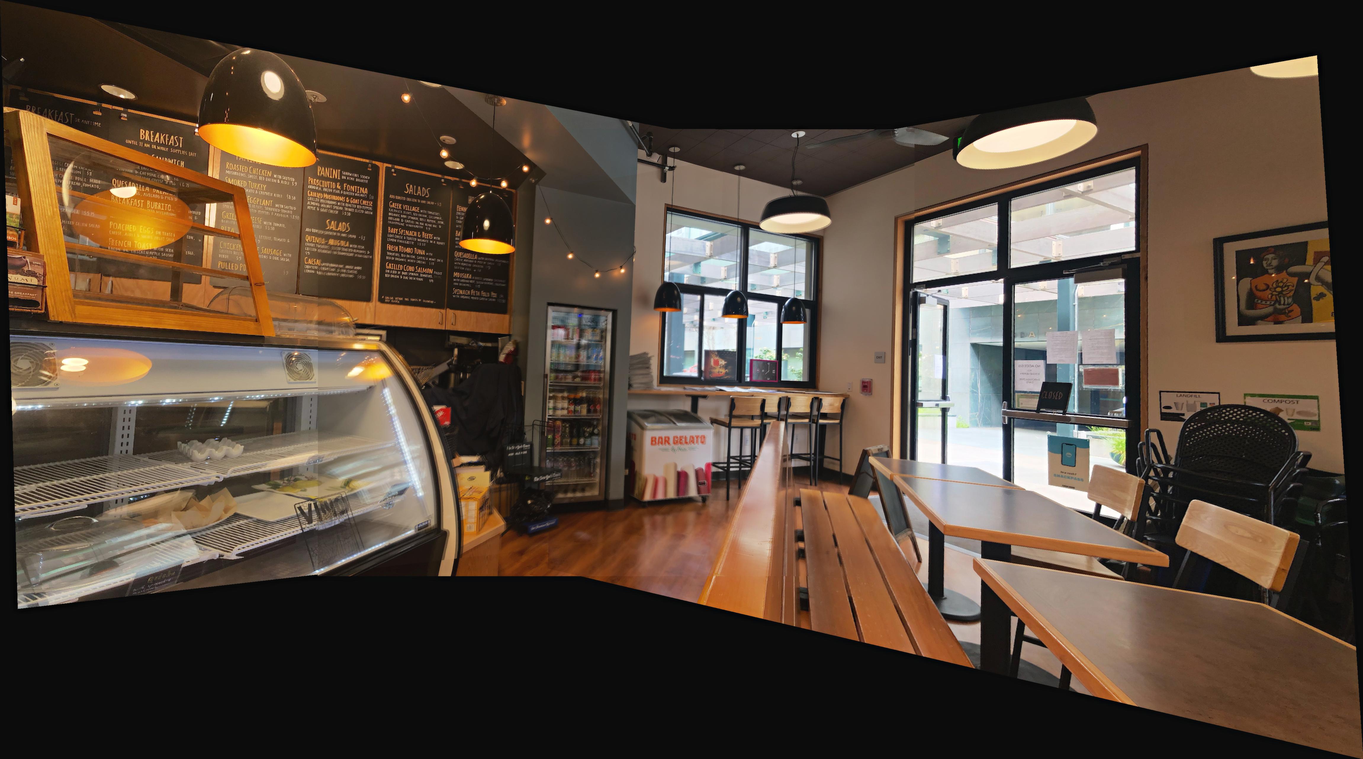
Below we compare the results of the manual and automatic method.

Manual	Automatic

Bells and Whistles

Video mosaics

We complete a video mosaic of a river with a length of 10 seconds. It can be viewed in Youtube below. To get a better view, you can set the quality to 2160p!

Reverse Rectify

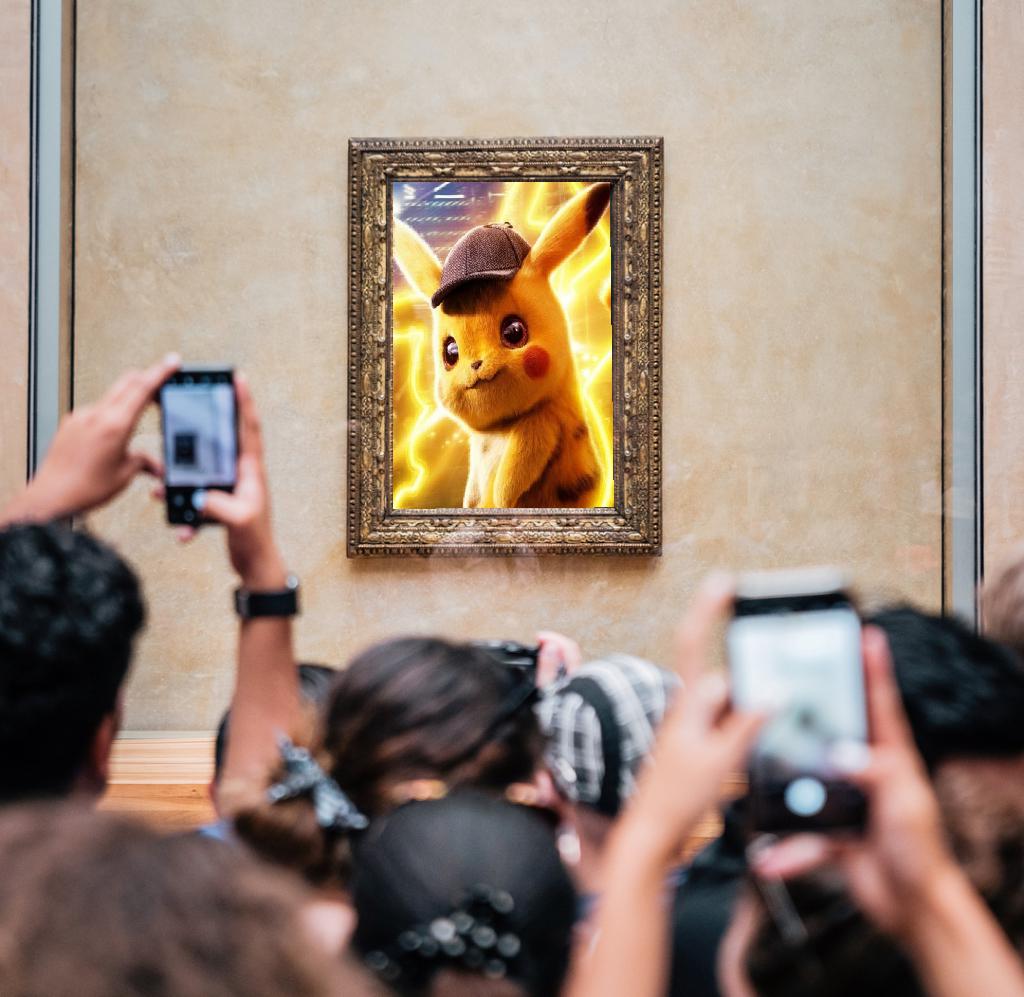
We can use the warping and blending technics to create some interesting images. Since we used to rectify the image in the previous part, we can also reverse rectify some photos into a new images. Below are some examples.

What I learned

Feature matching is the most amazing part in my opinion. I am always curious about how the computer can identify different features in images. I think it is cool by computing the distance of feature patches. Also, I found that making a panorama video is of great use to extend the capability of our camera. We can just get a magnificent time-lapse by just stitching several clips together!