CS194 Project 5
Image Warping and Mosaicing
Xuxin Cheng CS194-agv
Part 1 Image Warping and Mosaicing
1.1 Recovering Homogprahy
A Homography matrix is a 3x3 matrix with 8 degree of freedom. To solve this matrix, we need at least 4 pairs of corresponding points. If we have an overestimated linear system that has more than 8 equations, we can use Least Squares to solve this problem.
deliminate and combine other point pairs we can derive: , where h contains the 8 variables in homography matrix. Solving this least square problem we will have H, which is the homography matrix.
1.2 Image Rectification
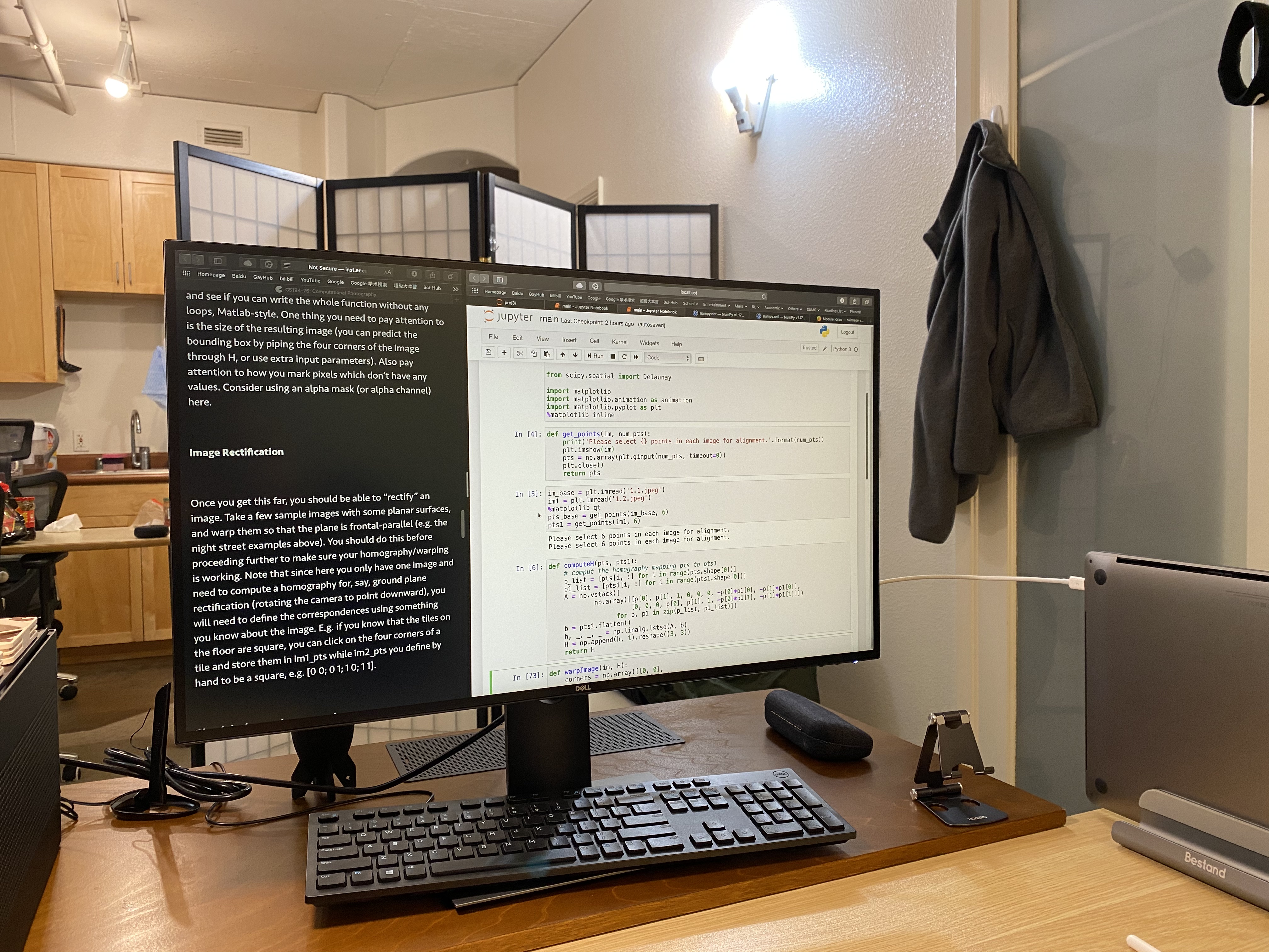 | 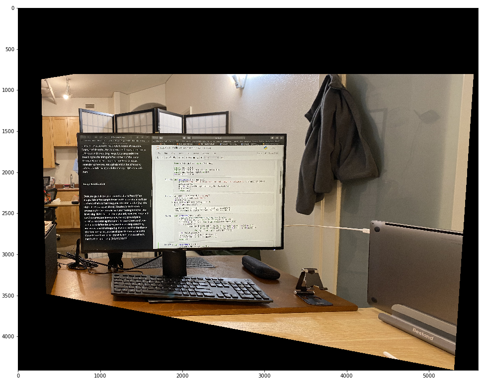 |
|---|---|
| original image | rectified image |
1.3 Blend the images into a mosaic
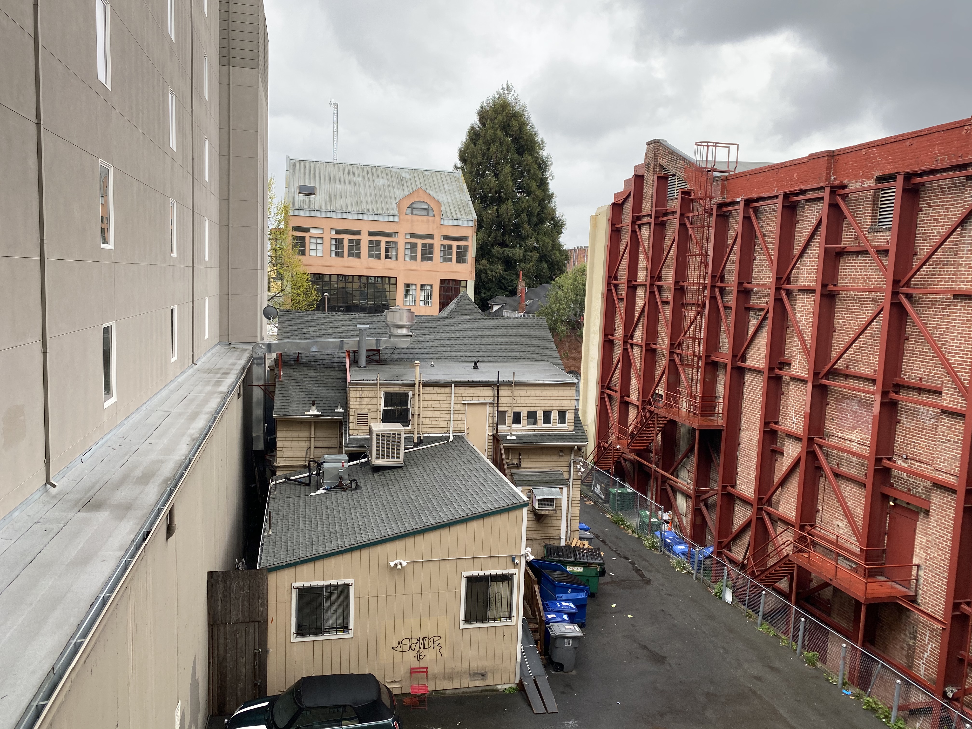 | 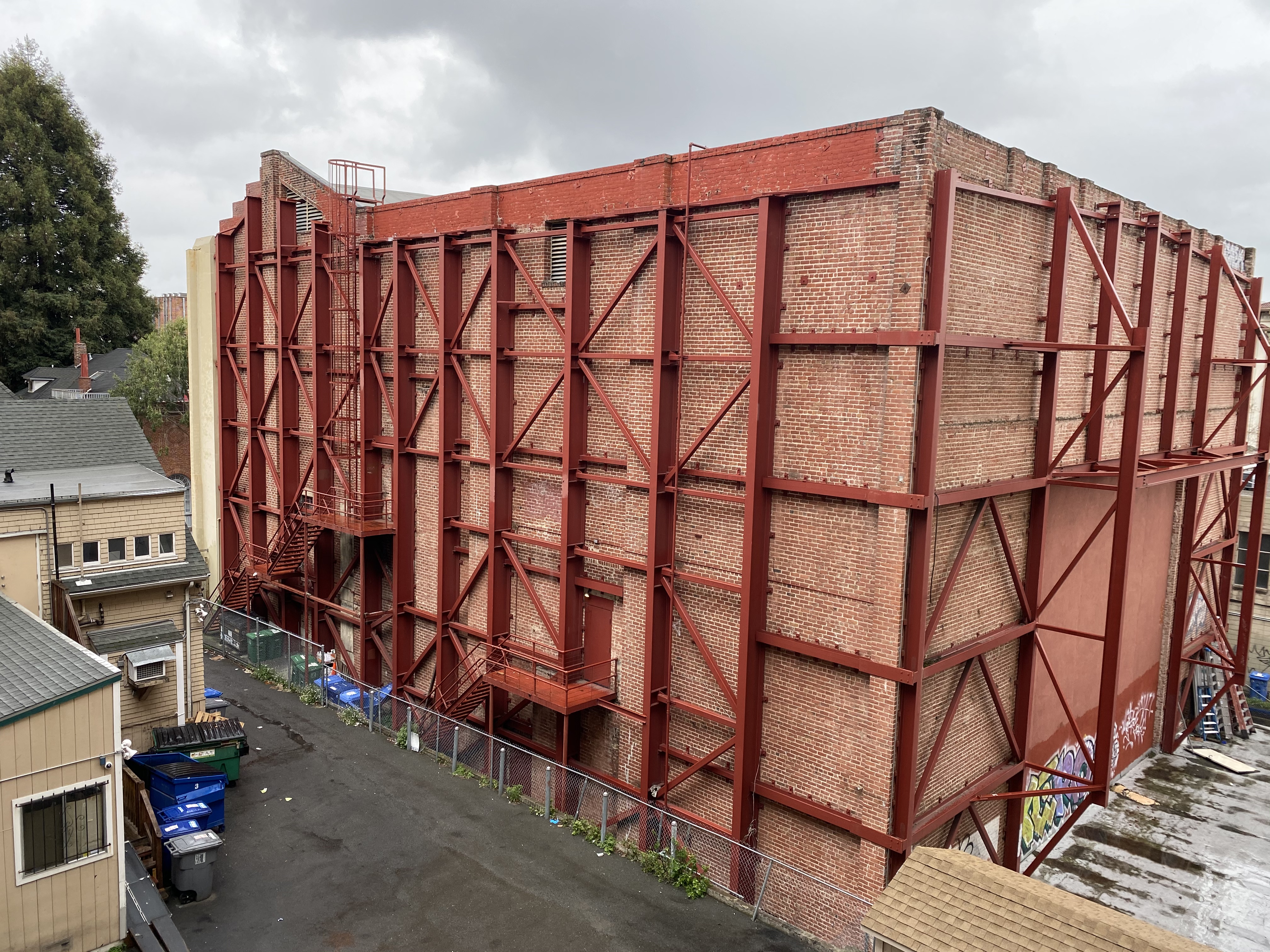 |
|---|---|
| image1 | image2 |
 |
|---|
| Blended image |
Part 2 Feature Matching for Autostiching
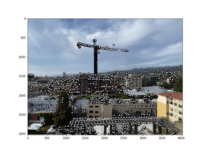
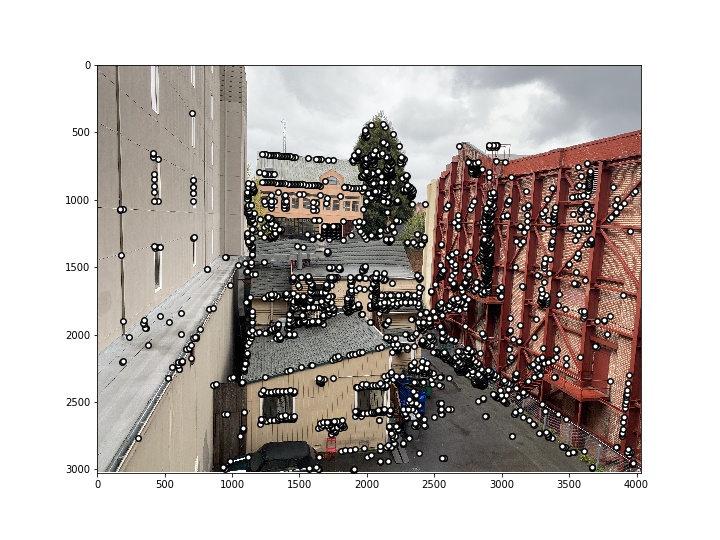
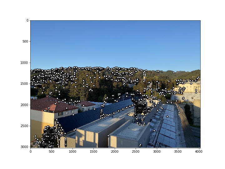
2.1Detecting corner features in an image
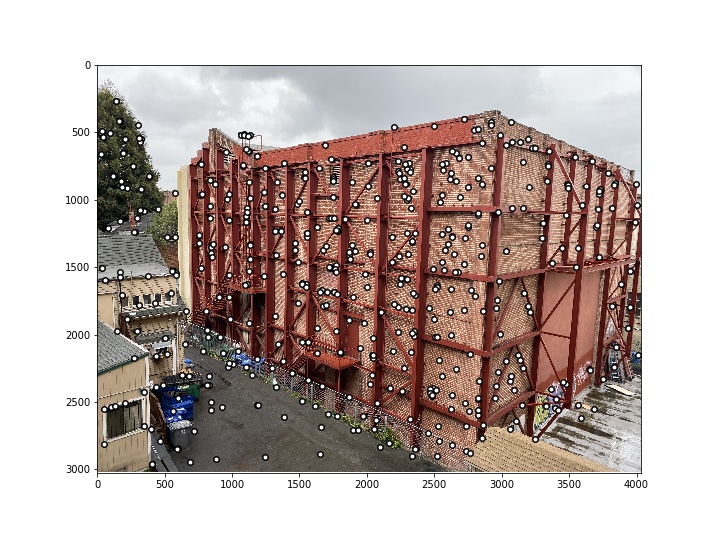
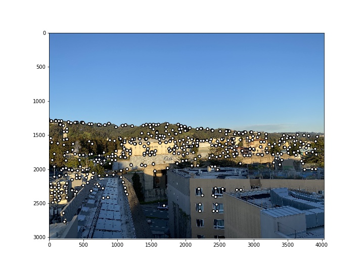
First we need to generate harris points. The points displayed are local maxima of R in a 1-pixel radius with a threshold of corner response 1. The extracted harris points are as follows:
 |  |
|---|---|
 |  |
 | 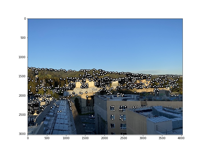 |
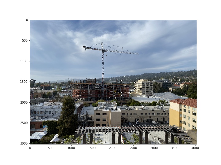
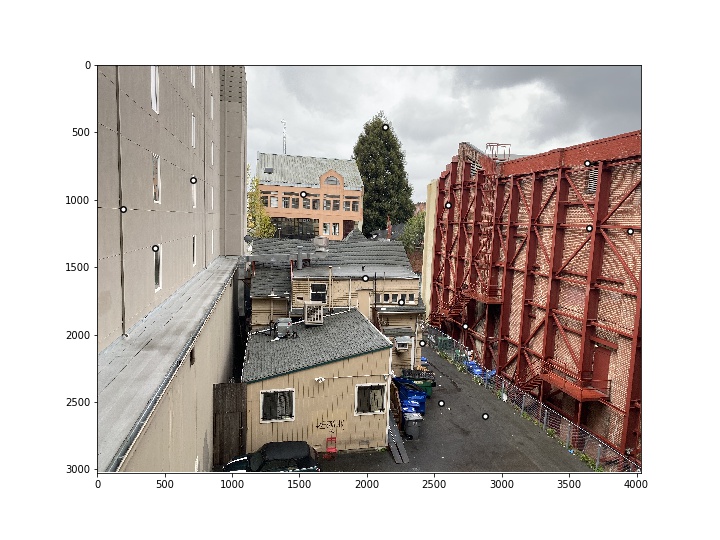
With Adaptive Non-Maximal Suppression (ANMS), we choose the best k points from the original harris points. Interest points are suppressed based on the corner strength , and only those that are a maximum in a neighbourhood of radius r pixels are retained. Conceptually, we initialise the suppression radius r = 0 and then increase it until the desired number of interest points n ip is obtained. In practice, we can perform this operation without search as the set of interest points which are generated in this way form an ordered list.

Here we choose and k=500. The results are as follows:
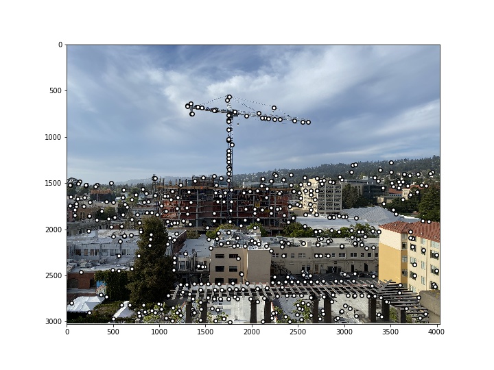 | 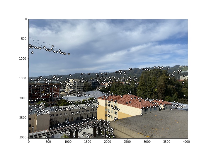 |
|---|---|
 |  |
 |  |
2.2 Extracting a Feature Descriptor for each feature point
Once we have determined where to place our interest points, we need to extract a description of the local image structure that will support reliable and efficient matching of features across images.
We need to Implement Feature Descriptor extraction. Here we ignore the rotation-invariance and just extract axis-aligned 8x8 patches from the larger 40x40 window to have a nice big blurred descriptor. Then we normalize the descriptors.
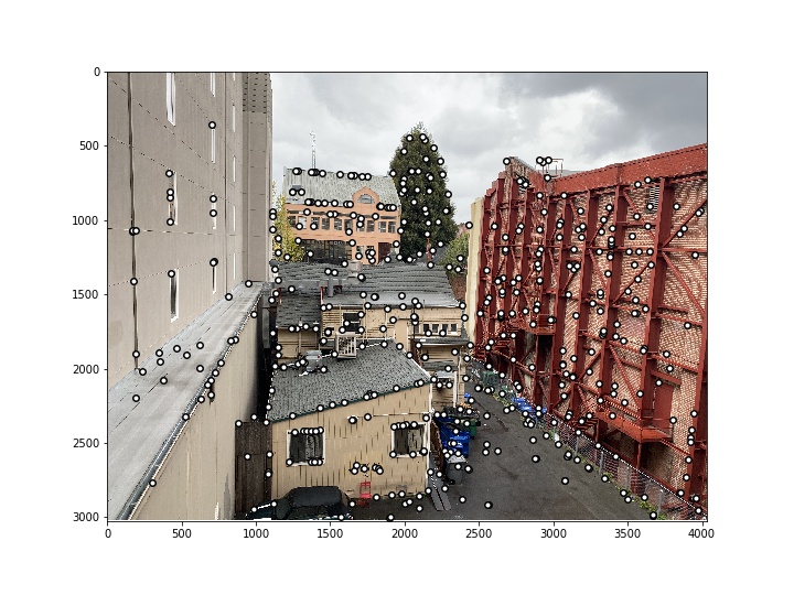
2.3 Feature matching
Then, each patch in the first image is compared to all in the second, with the criteria given by sum of squared differences (SSD) formula. Here we choose threshold . The results are as follows:
 |  |
|---|---|
 |  |
 | 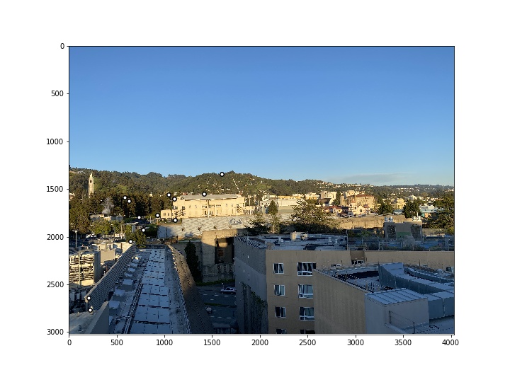 |
2.4 Use RANSAC to compute a homography
The last step is the Random Sample Consensus (RANSAC) algorithm to further reject outliers and get the best homography. We first choose four random pairs of matched points, then compute exact homography. Next we need to map all the remaining points of one image to the other and compute the corresponding SSD between projected points and real points in the second image. If the error is below 4, we count the point as an inlier. This process is iterated 10000 times, and the set of the highest number of inlier points is kept. The final homography is recomputed on this set of inlier points, and is used to warp one image to the other. The final points we use to compute homography are as follows:
 |  |
|---|---|
 |  |
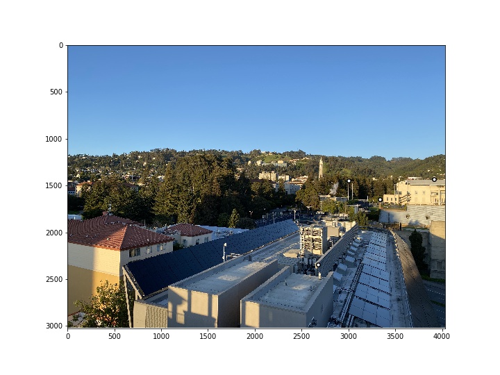 |  |
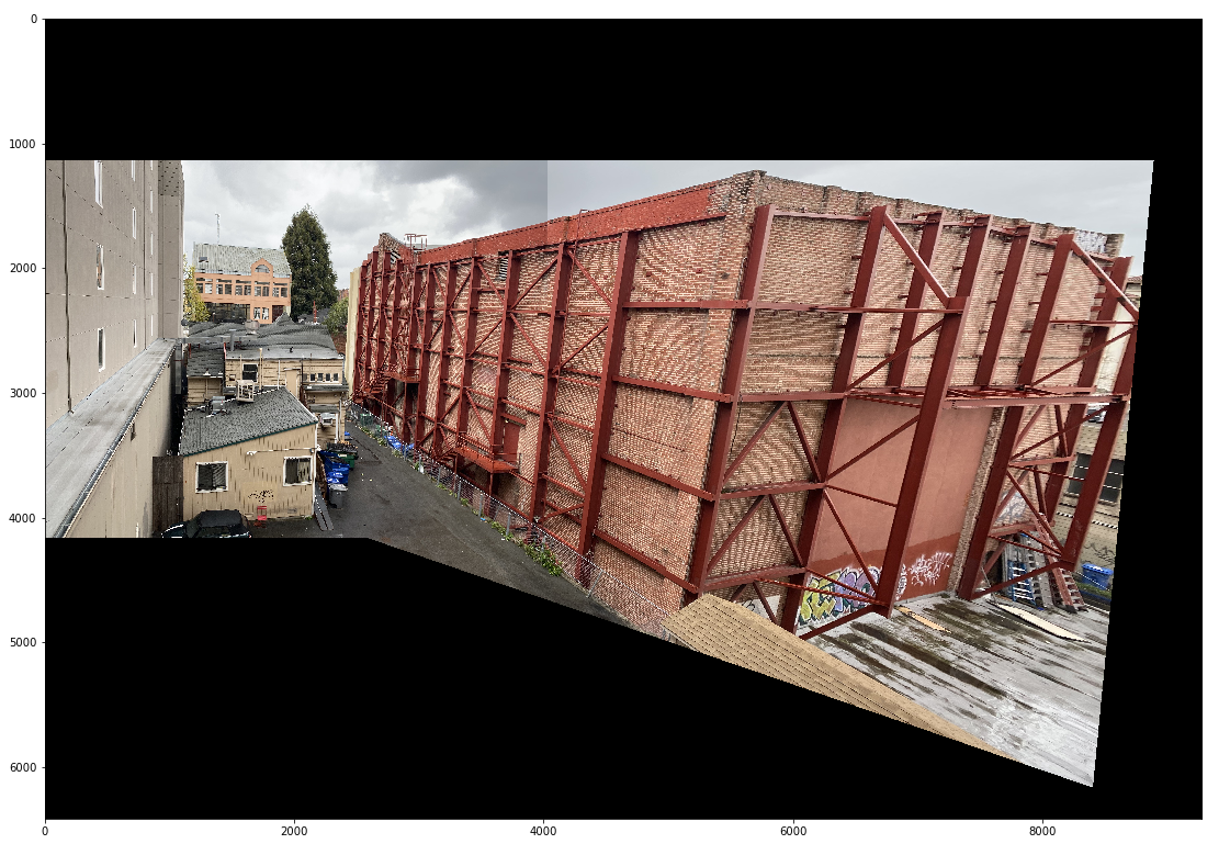
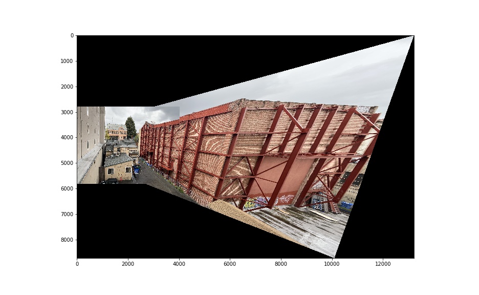
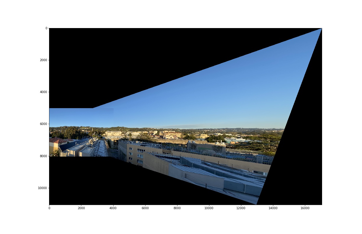
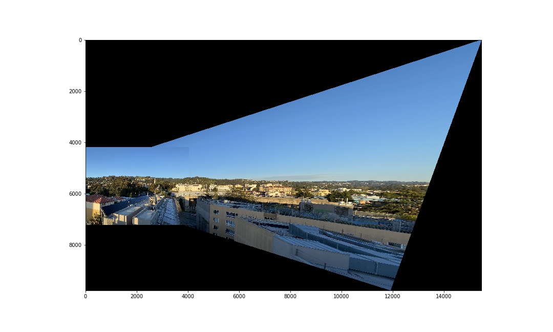
2.5 Produce a mosaic
We use the same method as in part 1 to compute an image mosaic.
| hand stiched | automatic stiching |
|---|---|
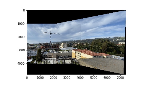 | 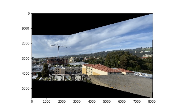 |
 |  |
 |  |
2.6 What I learned
From this project, I realized some so "hightechs" are actually from very simple ideas, which can produce amazing result without much effort. With 3 layers of filtering including ANMS, Feature Matching and RANSAC, we can actually pick 4 precisely match points from the the initial countless random points.