Proj5 Part1 IMAGE WARPING and MOSAICING

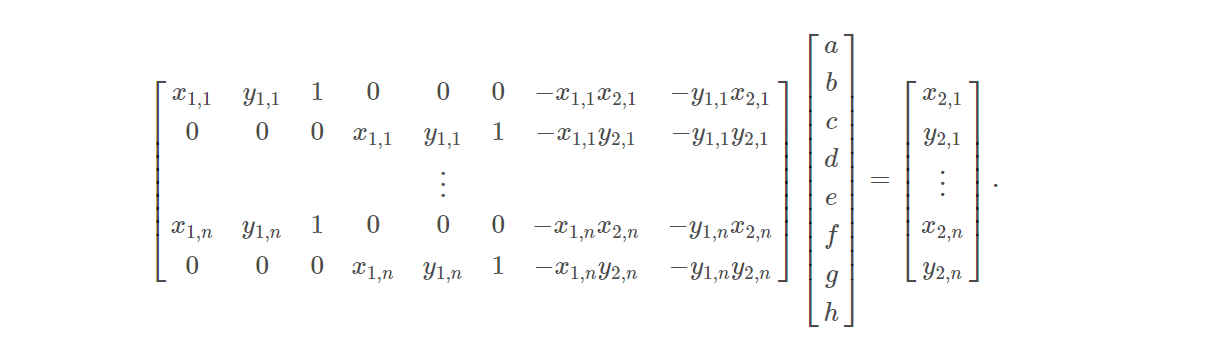
Recover Homographies

The least squre problem can be viewed in this form. But sovling this we obtain the transform matrix H.

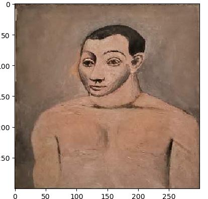
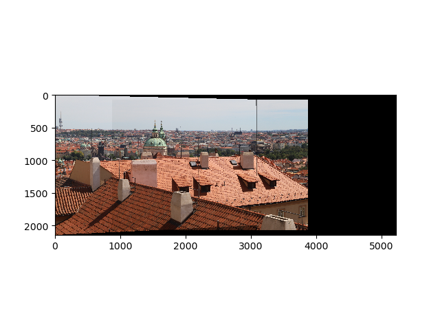
Warp the Images

After obtaining the transform matrix, we can use the similar method as in project3 to warp the pictures. By the mean time, I record the offsets from the unwarped picture for later procedures. Here are the examples of the rectified pictures

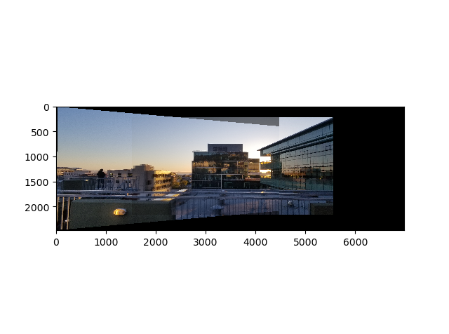
Blend the images into a mosaic

I blend the pictures one after another. And use the offset to track the position. At first I simply set alpha=0.5 But then I realize as the number of pictures increased, the first picture will be dimmer and dimmer.

Instead of using a mask, I want to try find the intersection and adjust it. So I find the intersection between the polygon of the two pictures to be blended. And divide the value of this area by 2. Other area just keep the original value. Since I blend the pictures by simply copy the value of the whole picture, the calculated intersection does not 100% represent the real intersetction. So we can see some darker area with straight edges. So use a mask to adjust the alpha channel will be a better and faster way. But I still choose to show this result.

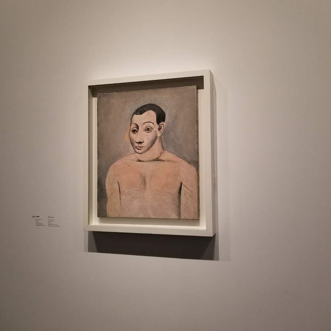
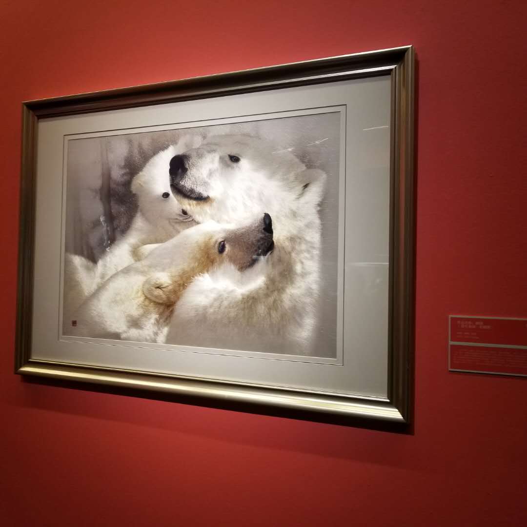
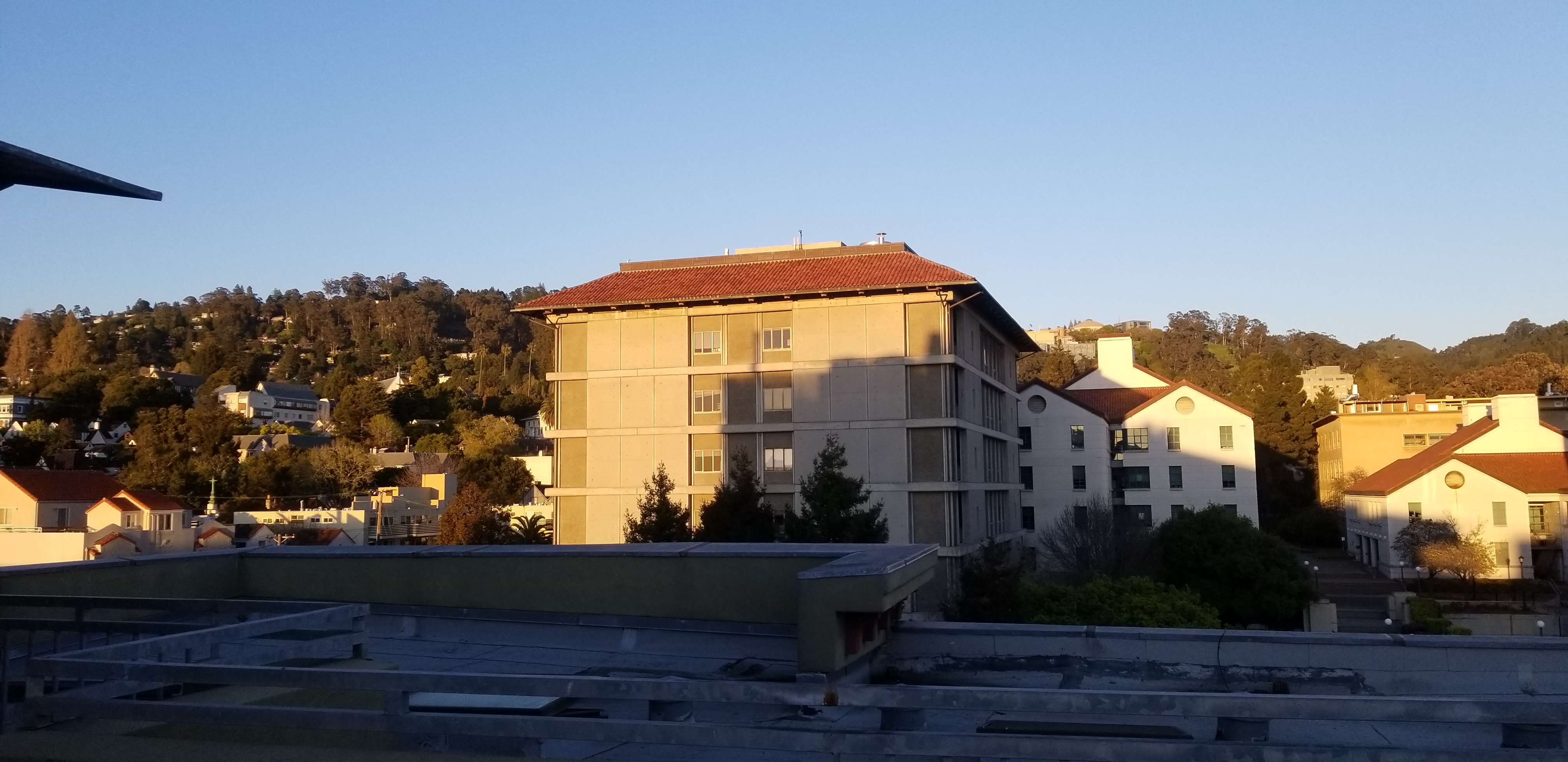
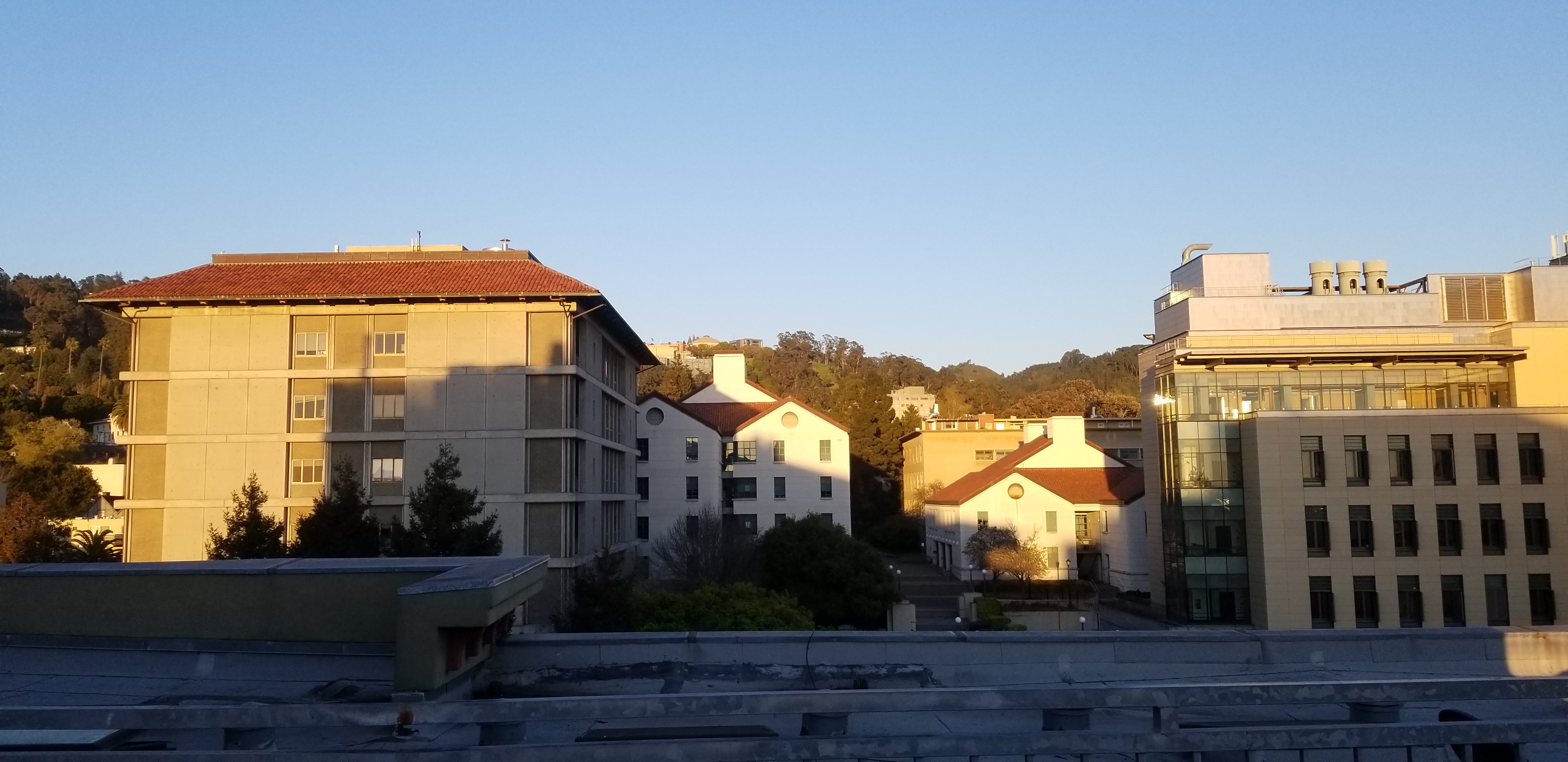
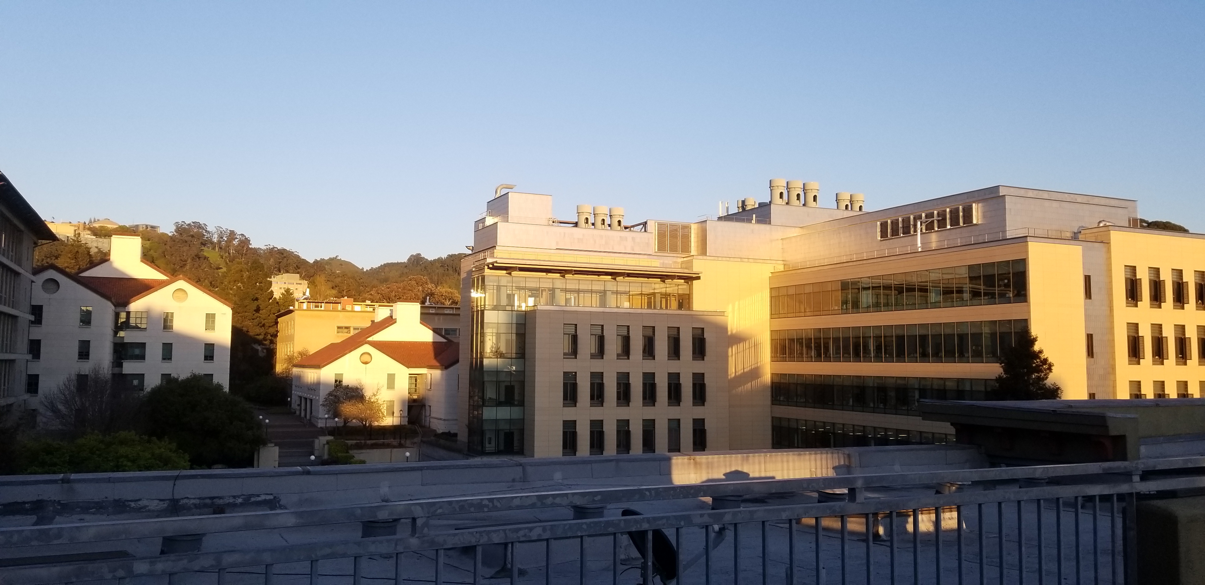
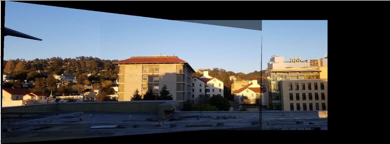
Original pictures:

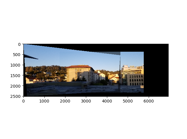
Coarsed result:

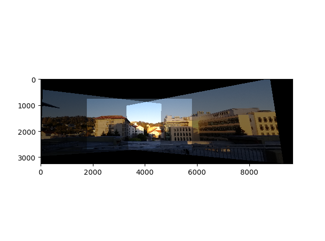
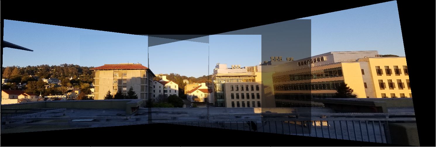
After adjusting:

What I learn

The point correspondance matters a lot. If I only mark point in just a certain area, the result is not good. So I need to spread the point evenly and include all the importan features. For better result, each picture need more than 15 points.

Proj5 Part2 FEATURE MATCHING for AUTOSTITCHING

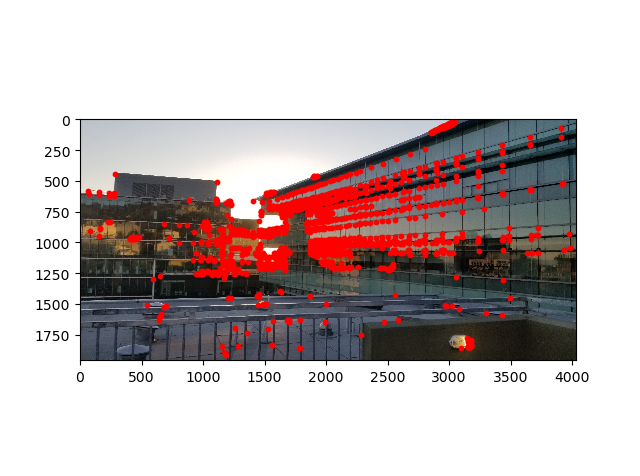
Detecting corner features in an image

Using the given get_harris_corners function we can get all the detected corner points. But we don’t need all this points, so we need to apply Adaptive Non-Maximal Suppression to get spatially well distributed local maximum points. The algorithm can be described as followings: 1. loop the points and find all the points with response bigger than 0.9*response(i) 2. calculate the distances with the all the other points. 3. set the biggest distance as i th point’s radium 4. find the points with biggest n radiums as the final output.

Before ANMS

After ANMS

Extracting a Feature Descriptor for each feature point

After obtaining points, we need to extract feature patch for further matching. We sample a 40*40 patch around the points then downsample it to 8*8 and normalize it.

Matching these feature descriptors between two images

To match patches, we calculate the distance between one patch and all the patches from the second image. If the 1NN/2NN is smaller, the likelyhood of correct matching is higher. Here we set the threshold as 0.4 as the paper suggested.

Use a robust method (RANSAC) to compute a homography

As we can see, there’re still many unmatched point. So we need RANSAC. The algorithm can be described as followings:

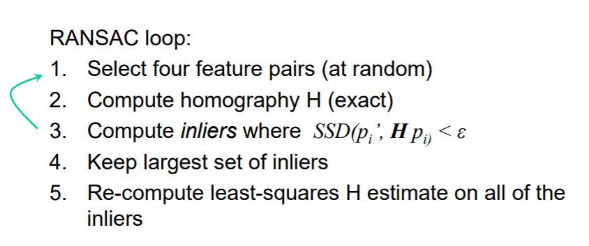
Here I choose 0.5 as the value of ε.

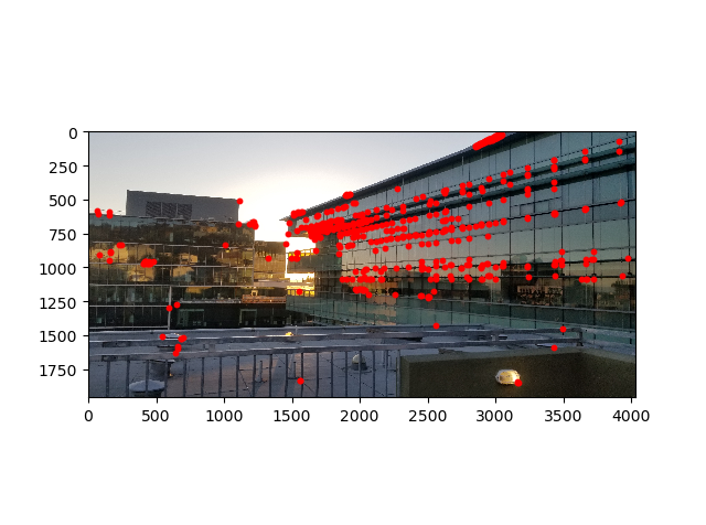
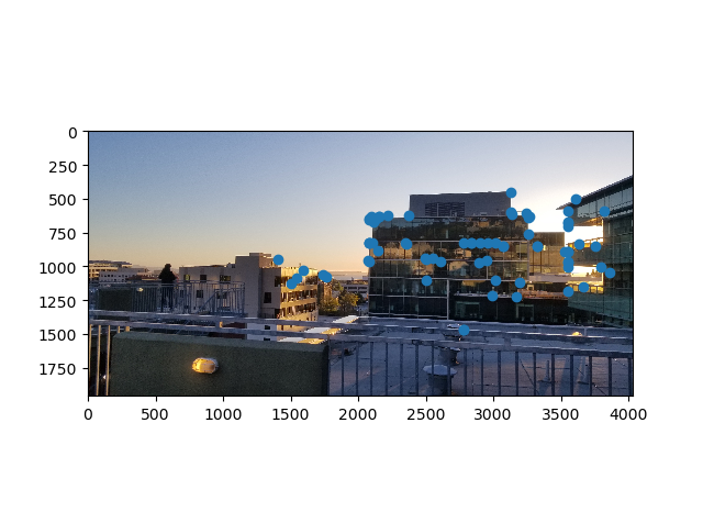
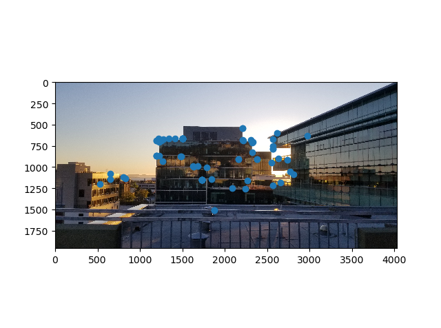
The final output matched points

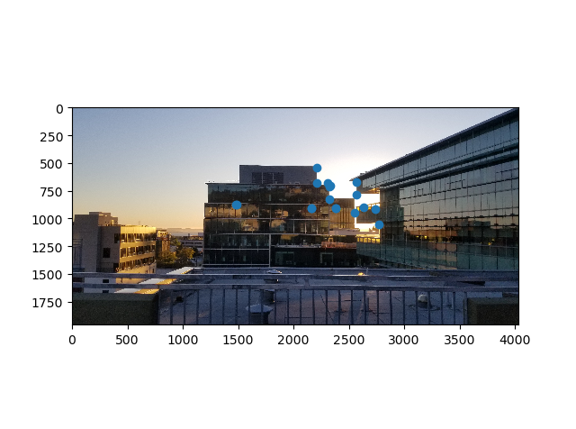
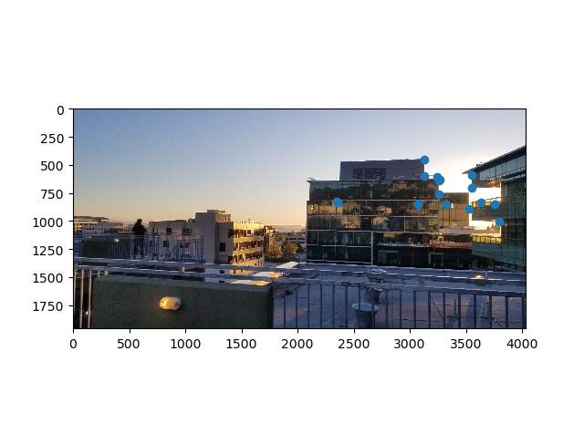
Three examples of autostitching

manual:

auto

What I learn

In order to get a perfect image using this pipeline, shooting buildings or other artificial stuffs will be a better idea. Since they tend to have obvious corners. On the contrary, the maximum detected harris points will tend to fall in the tree area which does little good to feature matching.