
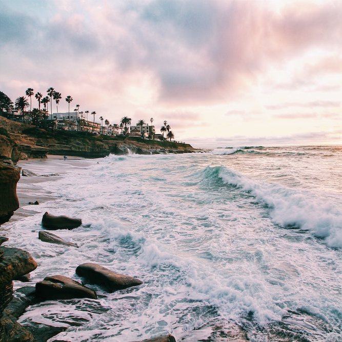
The goal of this project is to change image aspect ratios without warping or removing important aspects of the image. We define an energy function to determine which seams to remove.
Note: this algorithm works for removing column/rows of pixels; however, it does not mix the ordering as described in the paper. For this description, I'm going to assume attempting to shrink the width of the image i.e. we are finding and removing a vertical seam. The algorithm works the same way for shrinking the height.
The first thing we do is find the energy value for each pixel in the image. We used our Gaussian edge detector from project 2 for this.
We then want to find a vertical seam through our image that contains the least amount of energy. A seam is defined by a set of pixels where there is only one pixel per row and each pixel is only, at maximum, one pixel to the left or right of the pixel above. Seam finding is done with dynamic programming, starting from the top and working our way down, finding the least amount of energy to get from the top of the image to the target pixel. Here is an example of a minimum seam:
Once we remove the seam, we repeat the whole process of calculating the energy matrix and seam finding until we reduced our width to our target width.
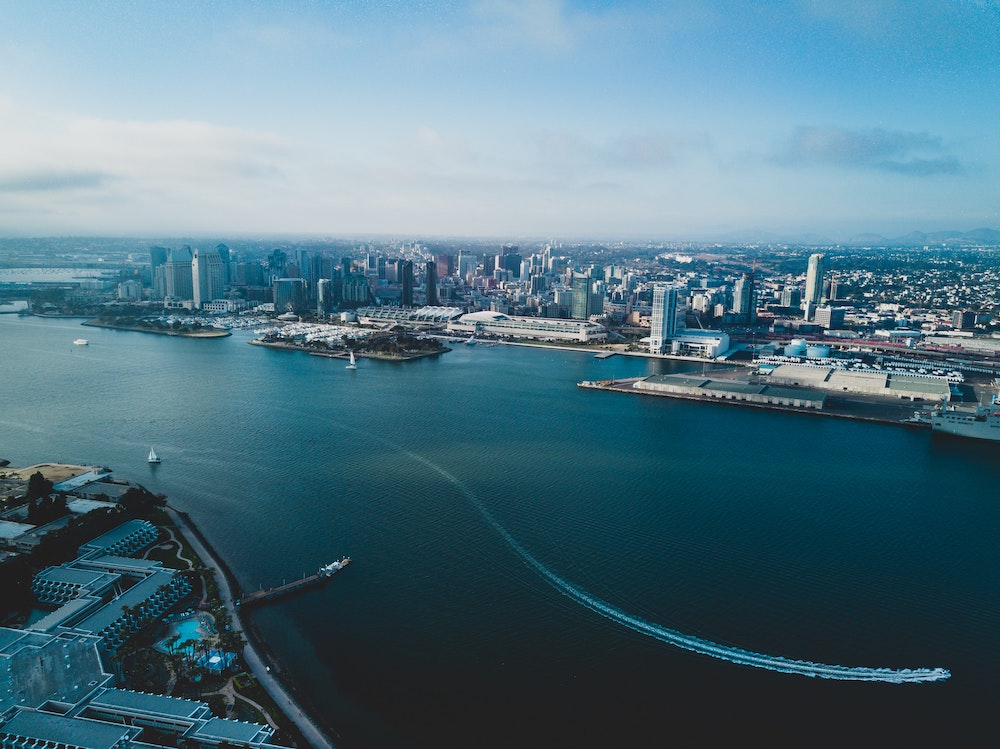
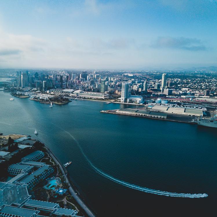
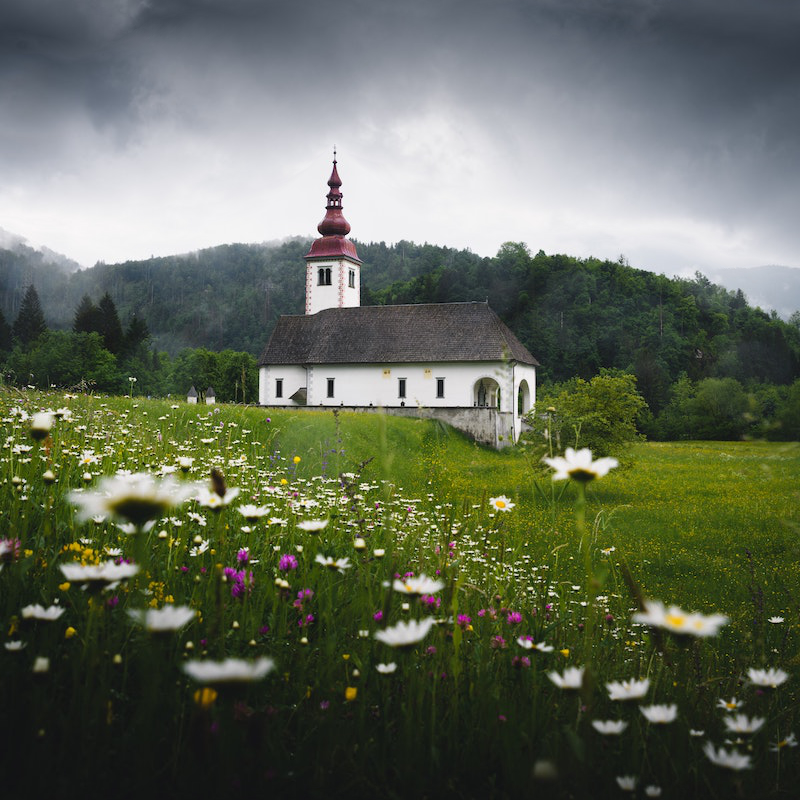
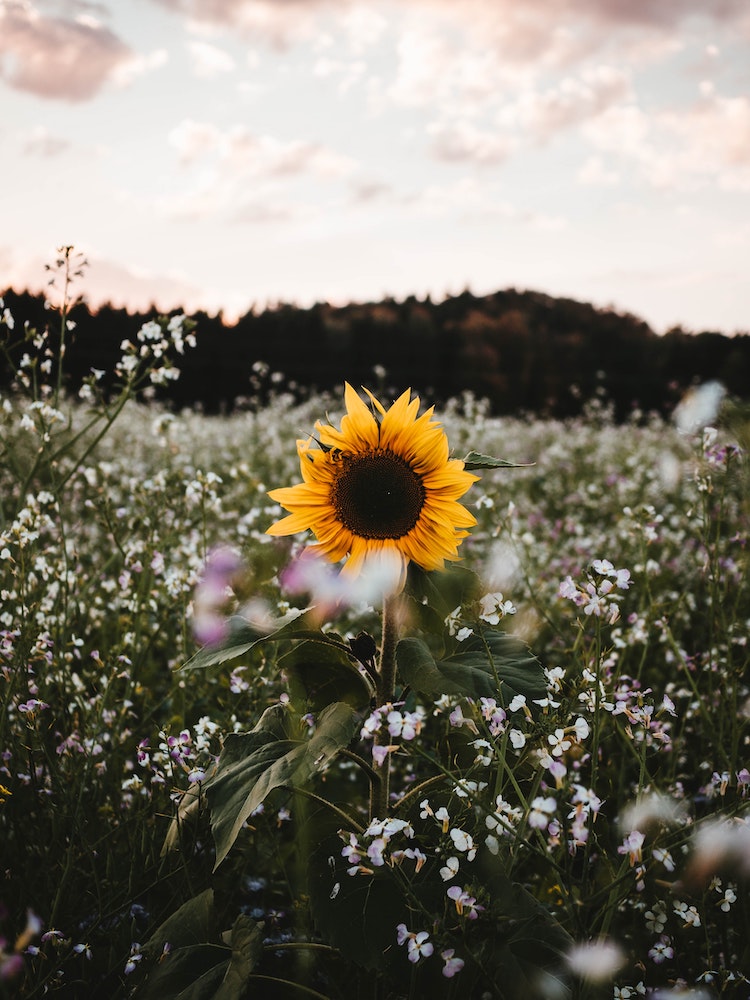
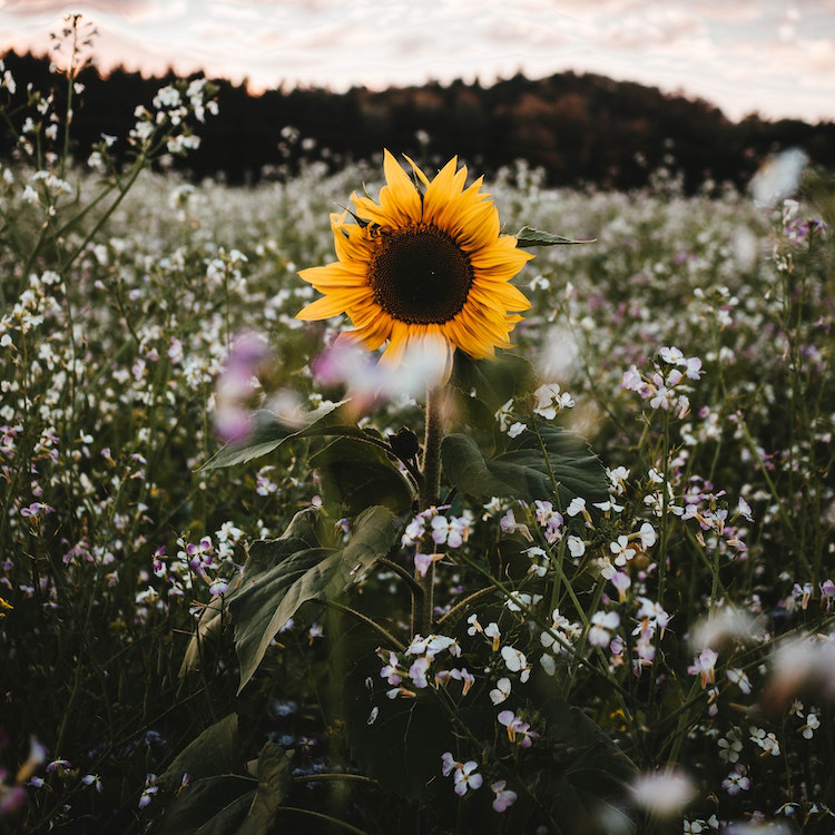
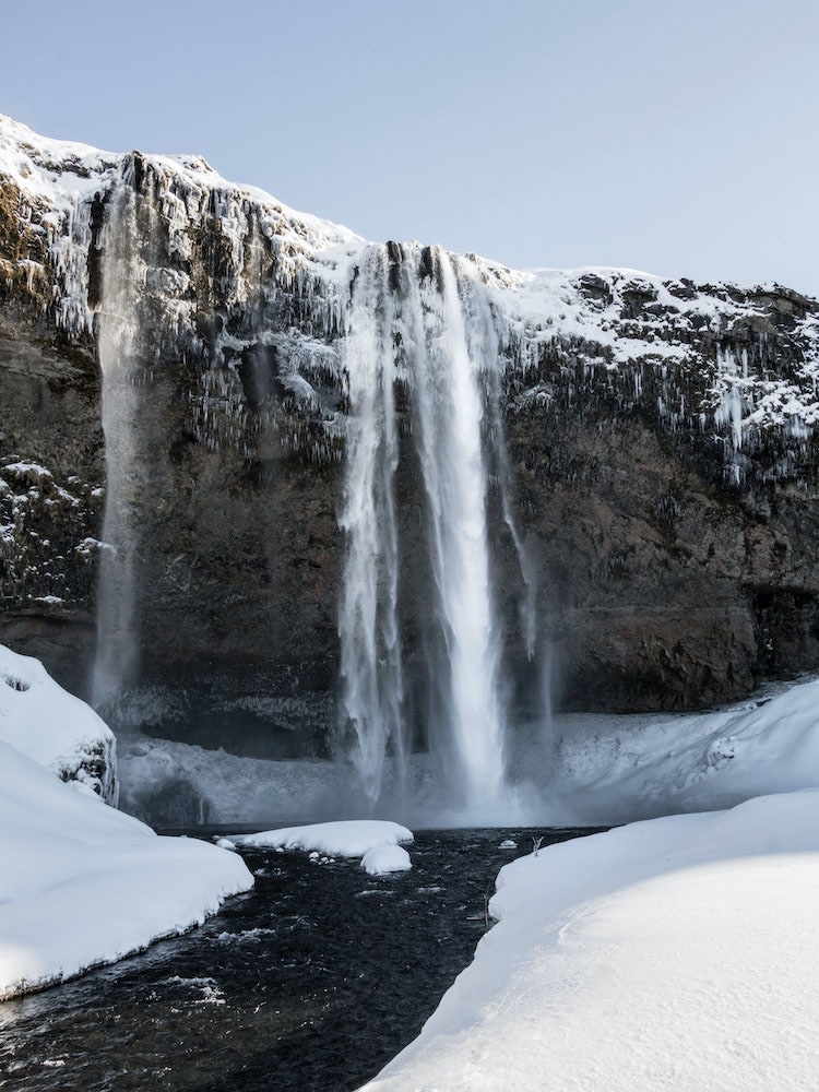
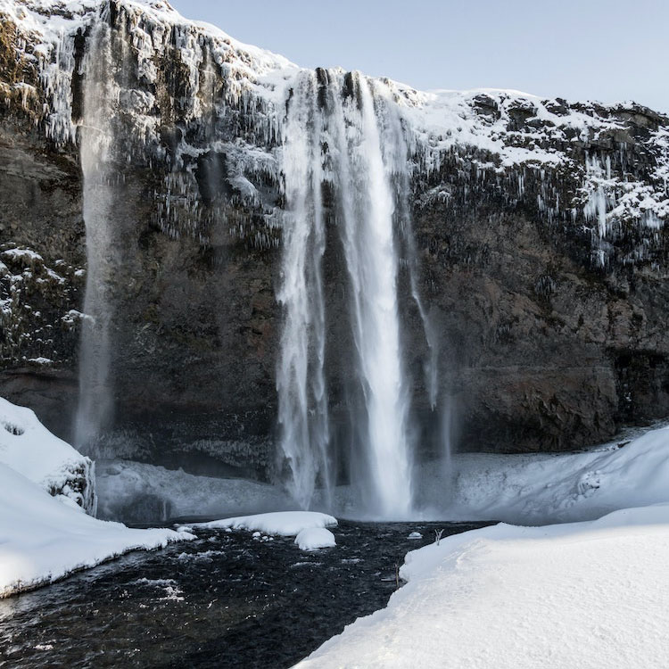
Here are examples of seam carving:
|
|
|---|---|
|

|
|
|
|
|
|
|
|
|
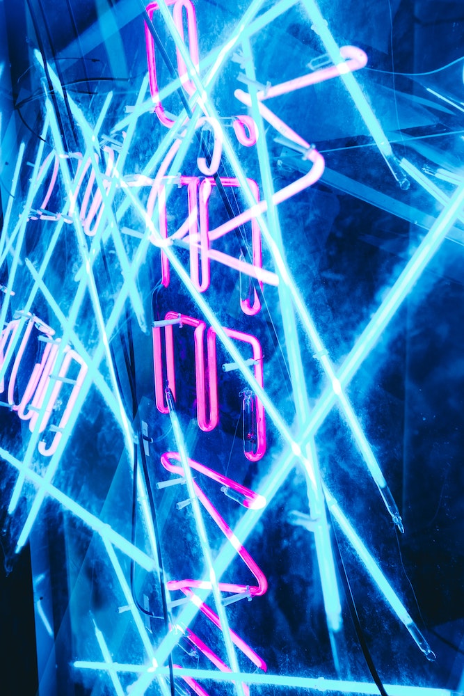
Here are a couple of failed photos.
|
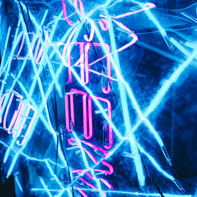
|
|---|
This one failed because there is an equal amount of information throughout the entire frame. The algorithm attempts to preserve the slope of the lights while removing parts of it, resulting is jagged edges.
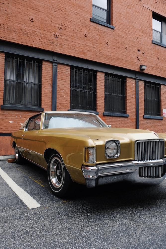
|
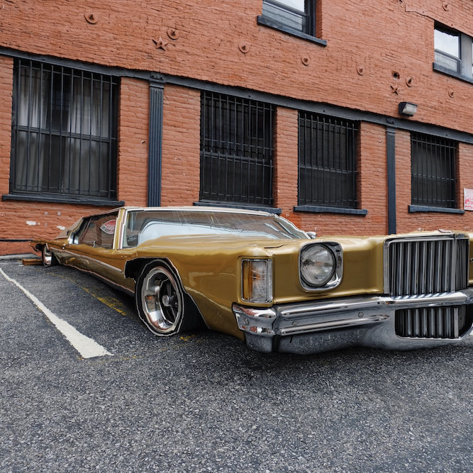
|
|---|
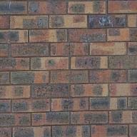
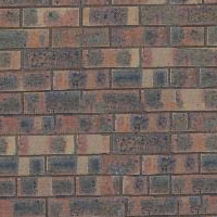
The car here is "smoother" than the wall in the background. As a result, the algorithm believes the car is less important and removes it before considering the wall.
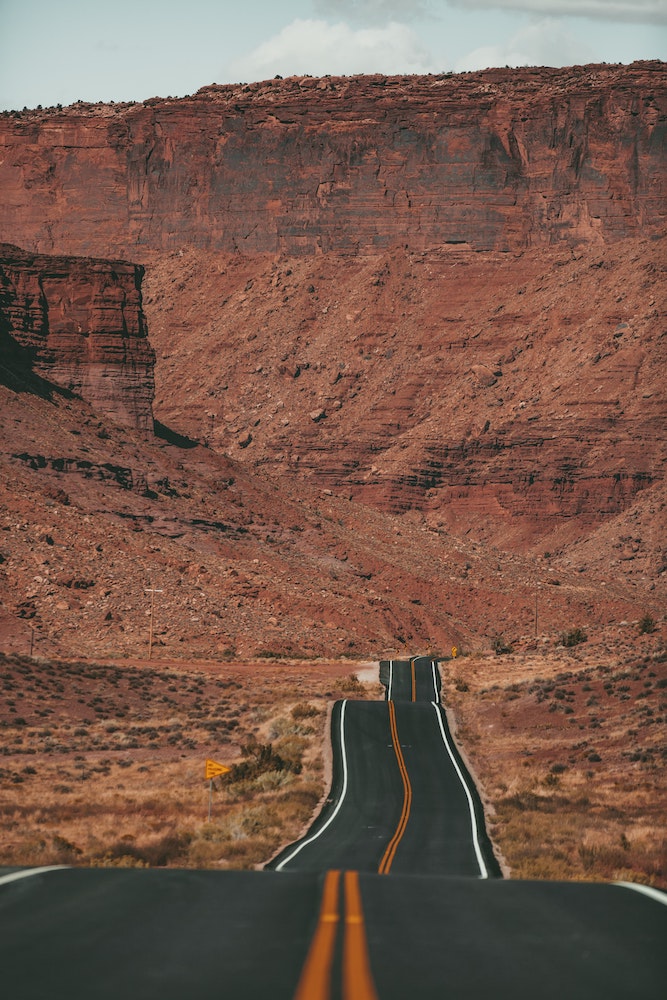
|
|
|---|
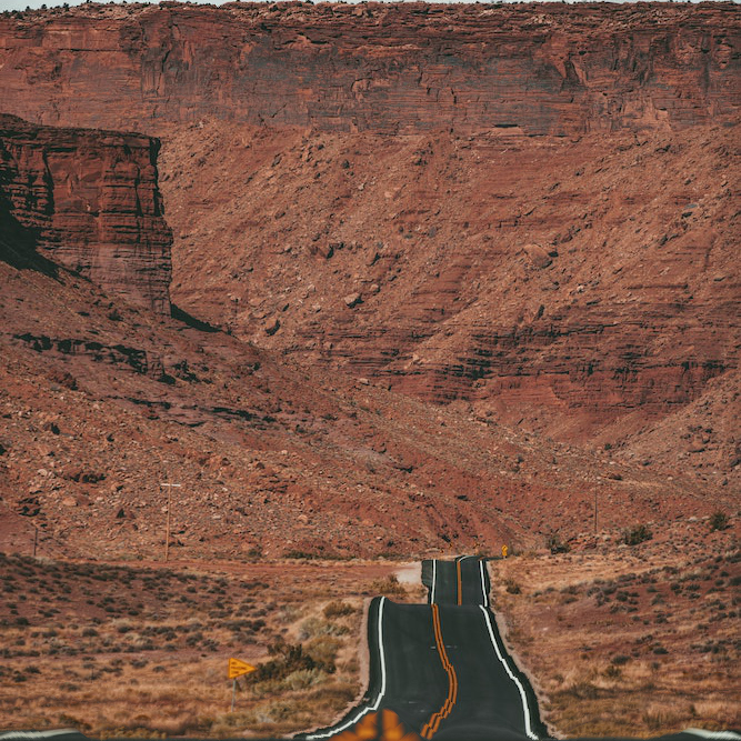
For the most part, this one worked. The only problem is in the foreground where we try to keep the blurred section of the lane divider without keeping the asphalt around it as the asphalt has low energy, resulting in the lane divider placed in the middle of the midground road.
We found it interesting how the algorithm what was considered high energy and what was considered low energy. While we know some parts of the image are part of the foreground, the algorithm does not, so if a smooth object is in front of a textured background, the subject will get removed first. This is probably something you have to consider when taking a photo that will be seam carved.
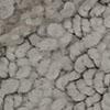
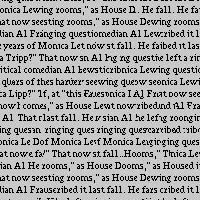
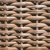
The goal this project is two-fold. We first want to be able to take a texture and simulate a larger image, or quilt, with the same texture. Once we can do that, we add a second criteria by comparing with a target image, allowing us to transfer texture from one image to another.
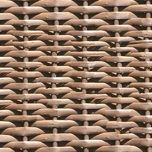
Throughout this project I will use the example text sample to perform quilting.
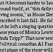
This is a very naive implementation where we just sample random patches of texture and place them side by side until the quilt is filled.
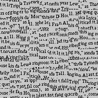
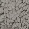
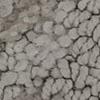
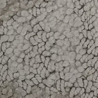
Instead of placing patches side-by-side, we now overlap the patches. We can use this overlap to evaluate image similarity and select patches that most closely resemble the quilt that is already selected. In order to include some level of randomness, we don't just select the patch with the smallest difference but rather randomly select a patch from the list of patches with a difference within some threshold (tol) of the smallest difference.
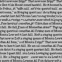
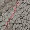
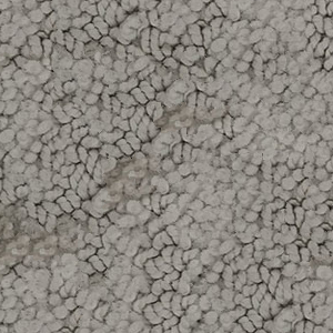
For seam finding, we implemented our own version of cut.m. We just used dynamic programming to find the min-cost cut from top to bottom by finding the minimum difference in value between the two images at every pixel. From there, it was just a matter of adding this function to the previous section's code so the transition between each patch is not as jarring.
In order to find a horizontal seam, we just pass in the images but transposed.
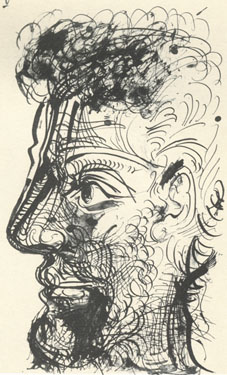
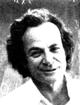
To demonstrate our implementation of seam finding, we're going to use two completely different images and visualize the seam it finds.
|
|
|
|
|
|
|
|
|
|
|
|
|

|
|
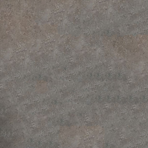
When finding the next patch, I added a second similarity check between the selected patch and a new target image. This new similarity and the original check are weight using alpha; I qualitatively selected alpha.
Below is the texture (left) I attempted to transfer to the target image (middle), and the result (right.
|
|
|
Here is a similar example but on an image of our own.
|
|
|
|
We implemented our own version of cut.m because there was no python version available (I cannot guarantee it is not the same as cut.m because I cannot read matlab code). The results can be seen in the "Cut Demonstration" section.
I have heard of style transfer in the context of machine learning but it is cool you can achieve similar results with just an algorithmic approach. This is much simpler and much more human-readable than the complicated networks needed for style transfer.
A very common scenario in photography is one where a camera is not able to capture the full dynamic rnage that exists in the target scene, leading to over-exposed sections, under-exposed sections, or a combination of both. With the objective of producing a single image that captures sufficient detail across the entire range, High Dynamic Range (HDR) is a technique for combining images captured from the same camera position across multiple shutter speeds/exposure times, such that the detail from each image is captured.
For this section, we look to recover a "radiance map" for a given scene from the set of multiple-shutter-speed images, largely following the steps detailed in this paper by Paul Debevec and Jitendra Malik.
When a camera takes a picture, it captures for each pixel a digital number, , that corresponds to an unknown function of the exposure
:
. Specifically, exposure is defined as the irradiance
multiplied by the shutter speed,
. Our general objective is to, given pixel values across the HDR set, as well as the shutter speeds, to compute the actual irradiance captured by the camera.
To make this objective more clear, we first apply the inverse of the unknown function to both sides, and then apply the natural logarithm to obtain the following:
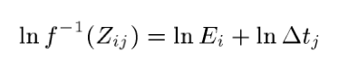
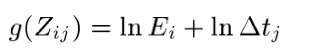
We define to be the function
, thus finally obtaining:
Thus, this becomes an optimization problem, where we'll use SVD to solve for the values of the function that minimize the following equation:
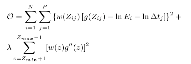
where...
In our implementation, we choose to sample the image in the middle of the image stack (usually has a shutter speed of 1), for each of the entire range of values (0 to 255), and record the value of that pixel across every other image in the same set. We then use SVD via Numpy to solve for the estimation of g for each value from 0 to 255.
After getting the estimation for the function g, we solve for the log of the irradiance for each value 0 to 255 by solving the following equation:
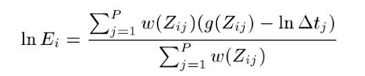
Our radiance map is then . For separate color channels, we do the above process for each color channel, and then combine them. In the case where the response curve/function
is fundamentally different for each color channel, we would have to find scalar terms, but for the images we tested on, the response curves are similar enough.
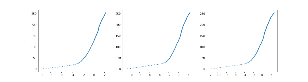
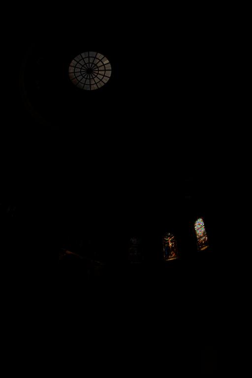
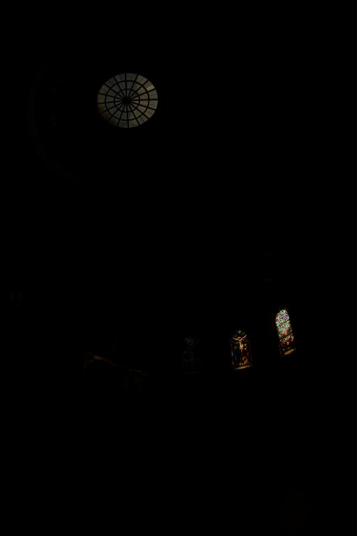
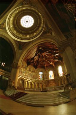
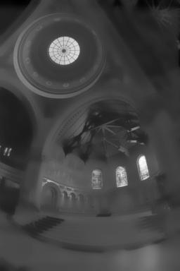
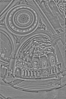
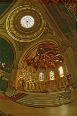
These are our results for the Stanford Memorial Church, which Debevec and Malik show in their paper.
|
|
The purpose of tone mapping is to in part ensure that the qualities of the image can be seen clearly. As you can see in the right-most radiance map in the previous section, much of the detail in the darker areas is still hidden.
Global tone mapping effectively adjusts the contrast of the entire image at the same time, allowing darker areas (or brighter areas) to be seen more clearly. However, since the entire image is adjusted at once, we cannot account for a wide dynamic range, which we can do with Local Tone Mapping. We'll show all our results in the results section below, and draw comparisons between them there.
While there are several choices for Global Tone Mapping, we choose to use Reinhard's tone mapping, where , for its ease of implementation and good results.
The alternative to global tone mapping is local tone mapping, which accounts for sections of the image individually, leading to better contrast results. The specific details of Durant tone mapping, which we implement, can be found in Durand 2002.
In general, what Durand tone mapping does is separate a given image/radiance map into two layers, the base layer and the detail layer. Then, contrast is altered (dynamic range is reduced) in the base layer, while the detail layer is preserved, thus allowing for previously-unnoticable detail to come through.
Separating the images into the base and detail layer is done via a bilateral filter. A bilateral filter is similar to a Gaussian filter, but has an added Gaussian component that accounts for color proximity - the larger the difference in pixel values, the lower the weight for that pixel becomes. It is in this way that the bilateral filter is able to achieve a smoothing effect without removing edges: edges differ significanly from their neighbors, so they both won't be accounted for in their neighbors' output, and also won't account for their neighbors in their output.
In our implementation of the bilateral filter, we precompute the spatial gaussian part of the filter, and manually compute the color gaussian component. We then iterate through each pixel in the image, applying the elementwise-product of the color and spatial gaussian term, normalized. This implementation is slower than ideal (Durand suggests several optimization methods), but we chose to continue with it in order to focus on producing HDR results instead.
With the bilateral filter, we follow the steps outligned in the assignment. The following directly builds off of the steps given, but we add notes on our implementation throughout.
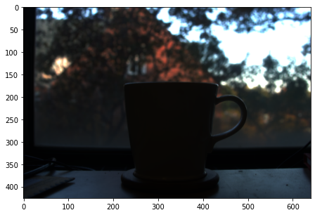
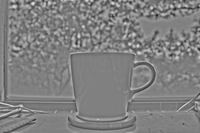
For each set, we provide the radiance map, the global tone mapping, the base and detail layer split via bilateral filter, and the final local/Durand tone mapping.
|

|

|
|

|
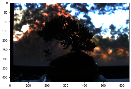
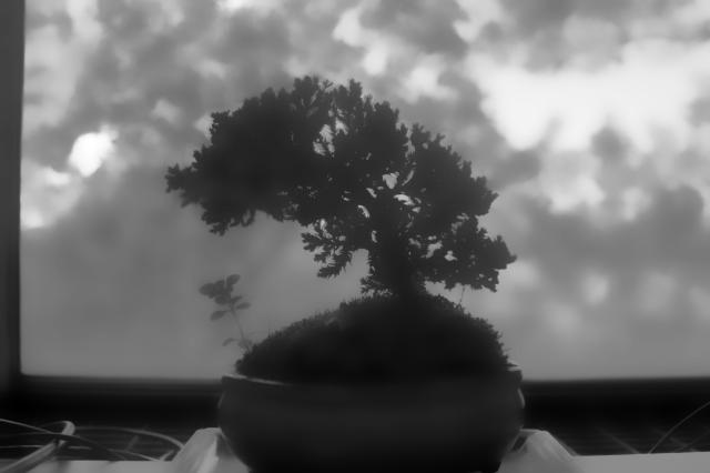
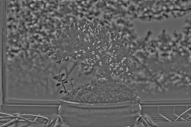
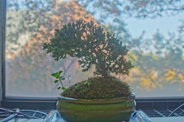
Note that in the Reinhard image, some details are visible, but those of the trees outisde the window are still blown out. In the Durand image, the cup is only slightly darker, but we can see those leaves clearly.
|
|
|
|
|
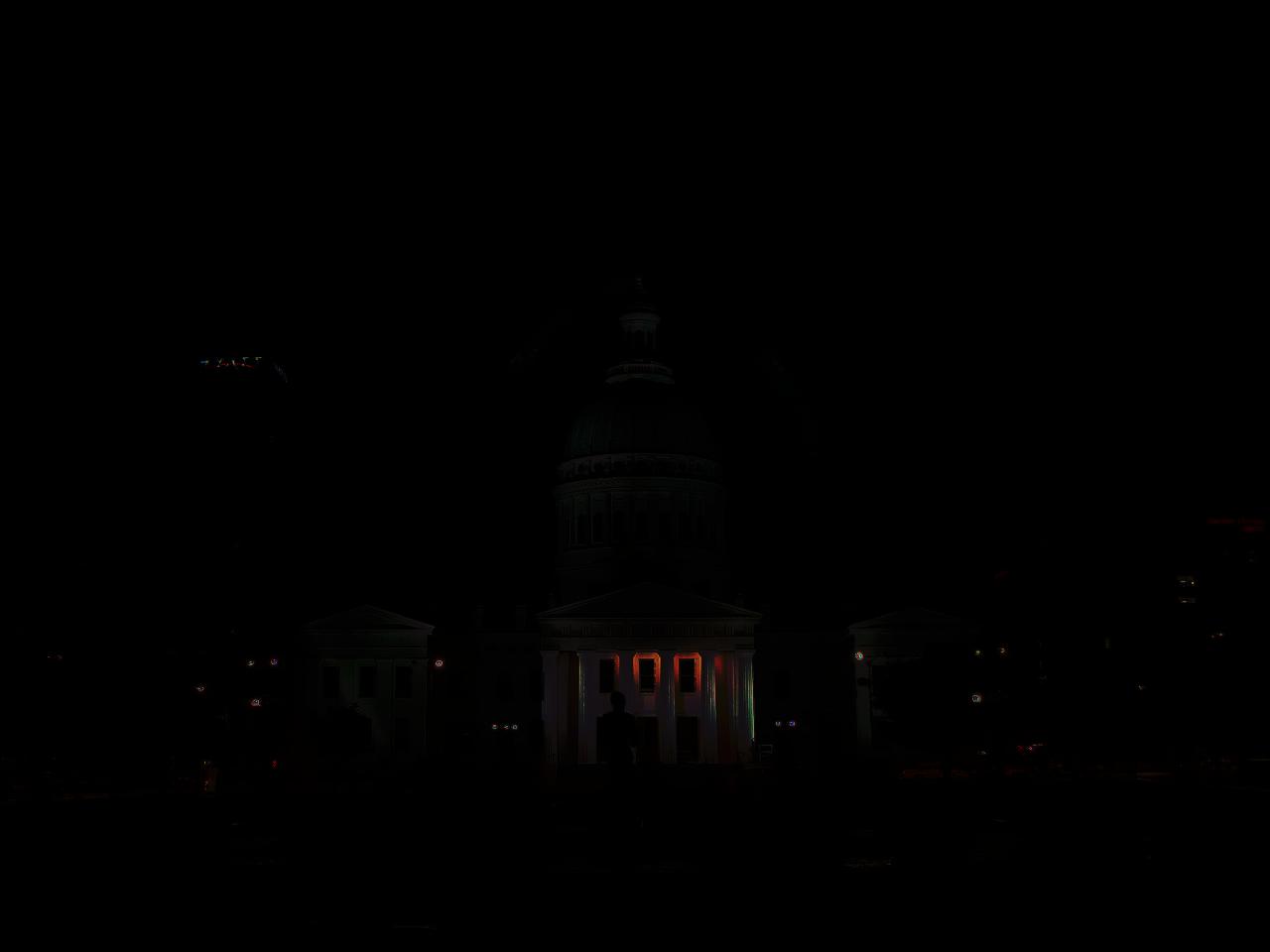
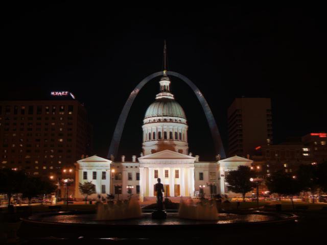
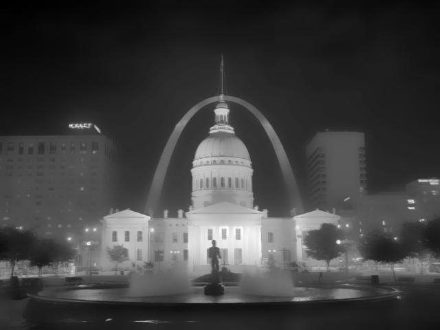
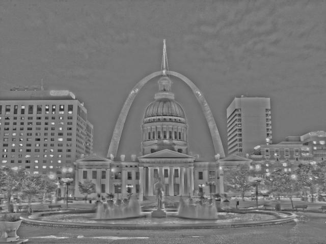
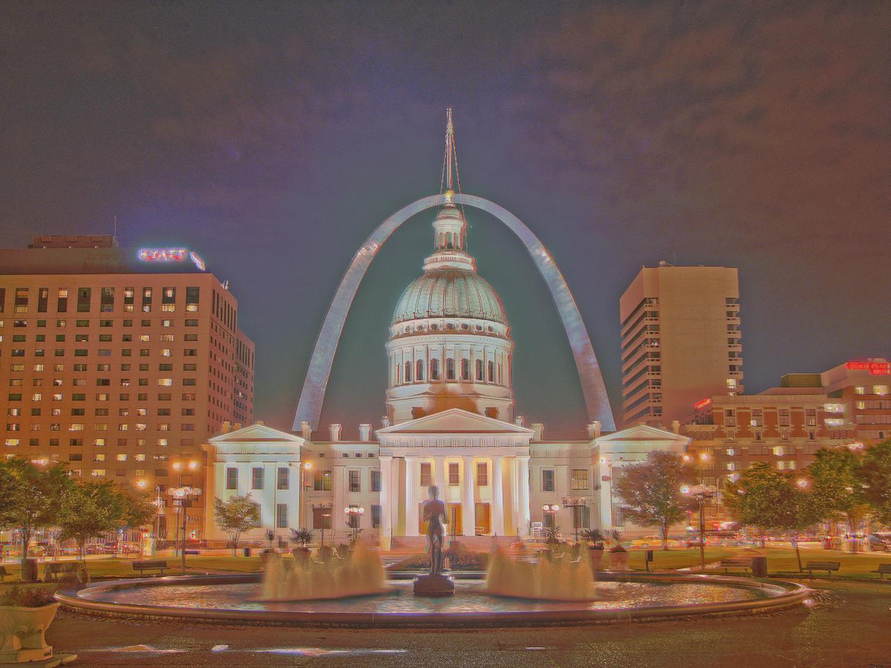
For the arch image set, we increased the Reinhard constant post-Durand tonemapping to make the details even more clear, at the cost of it seeming slightly washed out. We think it's a good example of the impact of parameters used. Nevertheless, many more details are visible with Durand tonemapping.
|

|
|
|
|
Pretty happy with these results.
|
|
|
|
|
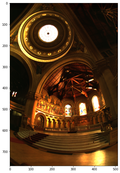
Church is an especially good example of how details can become visible in Local tone mapping that don't in global - notice the roof sections in the previously dark areas.
Overall, this project was a satisfying process of implementing an algorithm that we use quite often in day-to-day life. The underlying concept seems quite intuitive, but understanding the process, especially that in the Debevec paper, was very rewarding. Also, it's interesting to see the range of results in Durand tone mapping as a result of parameter selection.