Final Projects

CS 194-26 Image Manipulation and Computational Photography Spring 2020

cs194-26-aah

PROJECT #1: SEAM CARVING

In this project, I implemented the seam carving algorithm as described in Avidan and Shamir's Seam Carving for Content-Aware Image Resizing paper. The idea of seam carving is to successfully resize images while being content aware. Instead of rescaling or cropping an image, we instead want to remove 'seams' - a connected path from one side of the image to the other, choosing one pixel in each row (for vertical seam carving). The implementation is split into two parts:

1. Determine the importance of each pixel using an energy function.
2. Keep on removing lowest-important seam until desired image size.

Algorithm details:
The energy function I used was simply taking the sum of the derivatives in the x and y directions at each pixel. To find the lowest cost vertical seam, let e(r,c) be the energy at row r and column c, and let f(r,c) be a function that computes the lowest-cost path from the top of the image to pixel at row r and column c. Let f(r,c) = e(r,c) + min(f(r-1, c-1), f(r-1, c), f(r-1, c+1)). Thus this function uses the coordinates of the 3 pixels in the previous row adjacent to r,c to compute the shortest path. Once I computed f(r,c) on all pixels, I found the pixel in the last row with the smallest f(r,c) value. From there, I backtracked each row above to follow the adjacent pixel with the smallest f(r,c) value, keeping track of the index of each pixel to be removed. Once I reached the top of the image, I now had all the indices in each row that would produce my seam. I removed the seam with simple numpy operations.

Here are some rather successful results:

Vertical seam removal: 150 columns

Before	After

Horizontal seam removal: 90 rows

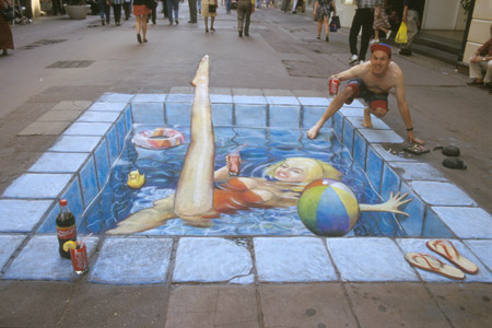
And here are some failures... I classified these as failures because I did not consider the resizing to be that content aware. For example, faces were either disproportional, vertical/horizontal lines in the image were not maintained properly, or there were noticable artifacts that would make your head scratch if you saw the image for the first time.

Vertical seam removal: 150 columns

Before	After

Horizontal seam removal: 90 rows

Project 1 Takeaways

The most important thing I learned in this project was how innovative even simple ideas are. The dynamic programming algorithm is very intuitive and therefore makes sense why it is a good approach at solving this resizing issue. While the algorithm I implemented was the naive version and could use improvements and optimizations, it's great that it could already provide me some successful results.

PROJECT #2: LIGHTFIELD CAMERA

Part 1: Depth Refocusing

The goal of this section is to refous at different depths afer taking the photos. I used the image set from the Stanford Lightfield Archive where images were taken from a 17x17 camera grid setup. Thus, each camera would produce images of the object from various angels.

The overarching idea of implementing depth refocusing is to first fix the coordinate location of a center image (in this case the coordinates of the middle camera at position (8,8), shift all other images to the center coordinates, and finally average the photos all together. To simulate varied focal lengths, I used an alpha value 'c' to adjust the shift offest. The equation I used to calculate the u,v shifts in the respective x,y directions was (u, v) = c * (cu - x, cv - y), where x and y are the coordinates of the current image, cu and cv are the coordinates of the center image, and c is the alpha constant.

Here are some examples of depth refocusing at different values of c.

c = -0.6

c = -0.2

c = 0

Here's a gif of the chess image with c = [-0.6, 0].

Here's some more examples on images of a crystal ball.

c = -0.6

c = -0.2

c = 0.4

Here's a gif of the crystal ball image with c = [-0.6, 0.6].

Part 2: Aperture Adjustment

This section plays around with simulating different aperture sizes. I used the implementation of shifting and averaging images in part 1 but this time with one limitation: radius. If sqrt(u**2 + v**2) < r, where u and v are the x,y offsets from the center image, and r is the aperture radius, then we include the current image in the subset of images to shift and average. With greater r, we can sample more images from different angles, letting more light enter the lens, simulating a greater aperture radius.

Here are some examples of aperture adjustment at different values of r.

r = 1

r = 5

r = 10

Here's a gif of the chess image with r = [1, 10].

Here's some more examples on images of a crystal ball.

r = 1

r = 5

r = 10

Here's a gif of the crystal ball image with r = [1, 10].

Project 2 Takeaways

It was cool to see how different alpha values play a roll in shifting the focus and aperture setting of an image. I've learned more about lightfield cameras in that they provide us more data to allow more complex post-processing effects.