import numpy as np
import matplotlib.pyplot as plt
%matplotlib inline
import skimage.io as skio
import skimage as sk
from glob import glob
from IPython.core.display import HTML
HTML("""
<style>

div.cell { /* Tunes the space between cells */
margin-top:1em;
margin-bottom:1em;
}

div.text_cell_render h1 { /* Main titles bigger, centered */
font-size: 2.2em;
line-height:0.9em;
}

div.text_cell_render h2 { /*  Parts names nearer from text */
margin-bottom: -0.4em;
}


div.text_cell_render { /* Customize text cells */
font-family: 'Georgia';
font-size:1.2em;
line-height:1.4em;
padding-left:3em;
padding-right:3em;
}

.output_png {
    display: table-cell;
    text-align: center;
    vertical-align: middle;
}

</style>

<script>
code_show=true;
function code_toggle() {
 if (code_show){
 $('div.input').hide();
 } else {
 $('div.input').show();
 }
 code_show = !code_show
}
$( document ).ready(code_toggle);
</script>
The raw code for this IPython notebook is by default hidden for easier reading.
To toggle on/off the raw code, click <a href="javascript:code_toggle()">here</a>.

""")
Lightfield Camera
In this project, we simulate depth refocusing and aperture adjustment with data from a lightfield camera: a camera that caputures both the intensity and the direction of light hitting the sensor.
I decided to use the "Lego Knights" dataset from http://lightfield.stanford.edu/lfs.html
Depth Refocusing
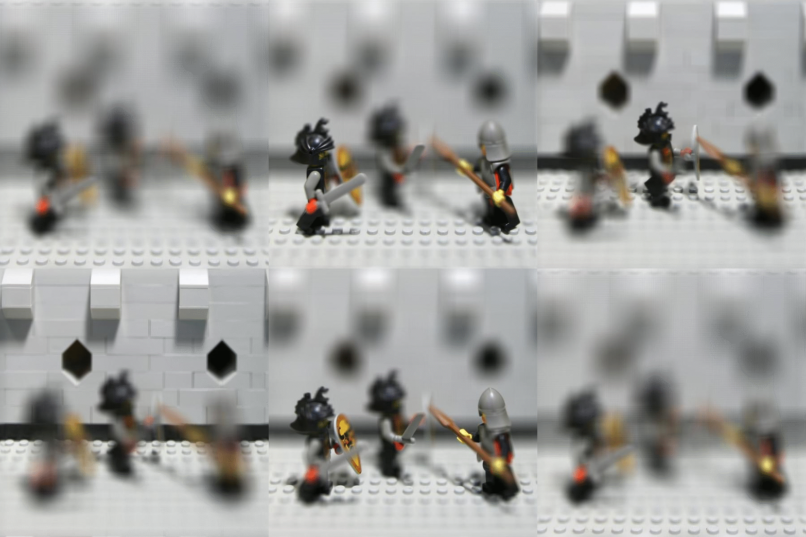
Because all of the images were taken from a 17x17 grid and evenly spaced, we can align the images to a central image by shifting one to another by calculating the offsets of the physical locations of the sensors. The actual depth is influenced by the scaling factor of the shifts. The overall amount to shift is calulated by shift = scaling_factor * (camera_loc[x,y] - camera_center[x, y]), where camera_center is the average x, y position for all of the images. By changing the scaling factor between -0.5 and 0.5, we can mimic different depths.
fig=plt.figure(figsize=(15, 15))
columns = 3
rows = 1
images = ["lightfield/depth/0.jpg","lightfield/depth/10.jpg","lightfield/depth/19.jpg"]
titles = ["front", "middle", "back"]
for i in range(0, columns*rows):
    fig.add_subplot(rows, columns, i+1)
    plt.title(titles[i])
    plt.axis('off')
    skio.imshow(images[i])
plt.show()
Gif

Aperture Adjustment
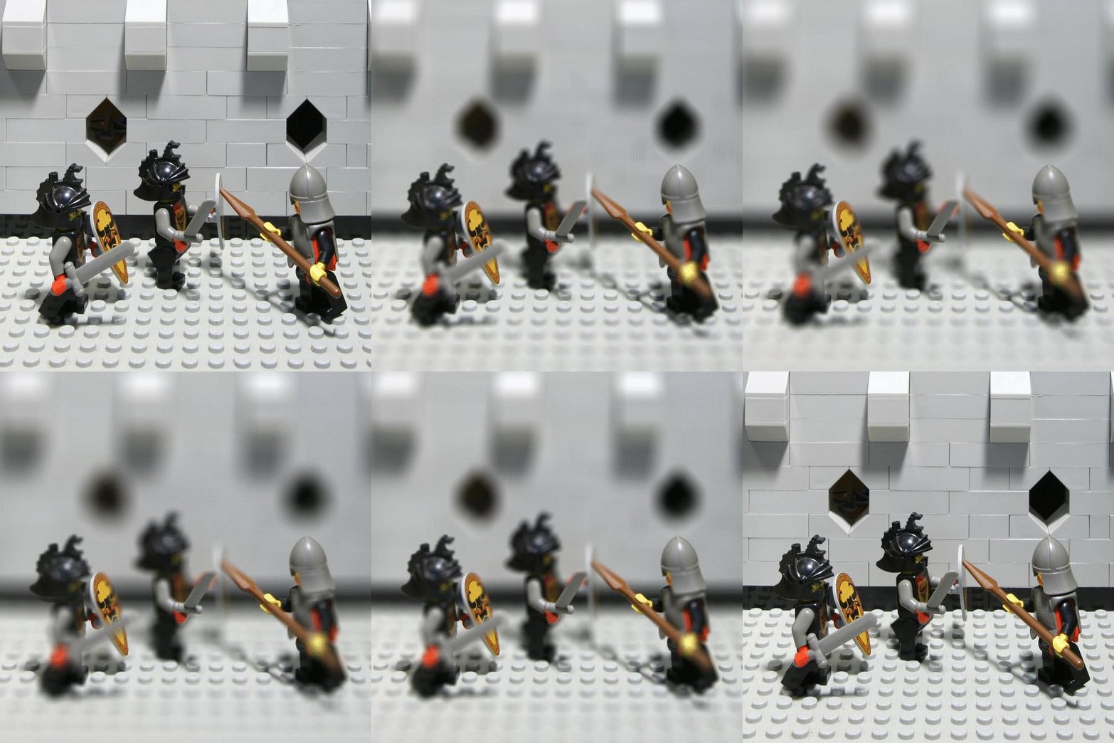
We can also mimic different apertures by averaging different numbers of images together. A small aperture (no depth of field) is simulated by averaging a small number of images together as there will be minimal blur outside of the where the camera is focused. However, averaging a large number of images will cause the images to be blurred outside of where the camera is focused, mimicing a large aperture (has depth of field). To get this effect, I varied the number of images to be averaged based on how close the images were to the central point (average of positions of the cameras). By using 1 to 289 (all) of the images, I captured the different apertures.
fig=plt.figure(figsize=(15, 15))
columns = 3
rows = 1
images = ["lightfield/aperture/0.jpg","lightfield/aperture/9.jpg","lightfield/aperture/19.jpg"]
titles = ["1 image", "137 images", "289 images"]
for i in range(0, columns*rows):
    fig.add_subplot(rows, columns, i+1)
    plt.title(titles[i])
    plt.axis('off')
    skio.imshow(images[i])
plt.show()
Gif

Summary
This project made me understand aperture and depth of field better, as well as how lightfield cameras work. It was really cool to be able to reconstruct a perfect picture (in terms of focus) from a bunch of pictures from a lightfield camera. It was also interesting to find out that just aligning the images doesn't impact where the image is focused, but you need to scale how the images are aligned.
Seam Carving
In seam carving, we try to resize an image by preserving the "interesting" parts of it. To do so, we must find a seam (a path from the top of the image to the bottom of the image that can only move straight down or diagoally 1 pixel to the left or right) with the lowest energy. We keep removing seams with the lowest energy until we reach the desired image size.
Energy Function
The energy function is taken from this paper, which is simply the sum of the abosulte values of the x, y gradients of the image: $\text{energy}(I) = |\frac{d}{dx}I| + |\frac{d}{dy}I|$. This measures how different the color of the pixels are in the x and y direction, allowing us to find a seam where the colors of its neighbors change the least (un-interesting).
Finding a Seam
We first generate a cumulative energy path (vertical) for every pixel on the top row using dynamic programming. Then, we find the bottomost pixel with the lowest cumulative energy, and then backtrack to the top to find the seam.
Horizontal vs. Vertical
The implementation for horizontal carving just transposes an image and then runs it through the implementation for vertical carving
fig=plt.figure(figsize=(12, 12))
columns = 2
rows = 3
images = ["seam carving/palm.jpg","seam carving/palm_carved.jpg","seam carving/sunset.jpg","seam carving/sunset_carved.jpg", "seam carving/seurat.jpg","seam carving/seurat_carved.jpg"]
for i in range(0, columns*rows):
    fig.add_subplot(rows, columns, i+1)
    plt.axis('off')
    skio.imshow(images[i])
plt.show()
Horizontal
fig=plt.figure(figsize=(12, 12))
columns = 2
rows = 3
images = ["seam carving/london.jpg","seam carving/london_carved.jpg","seam carving/stonehenge.jpg","seam carving/stonehenge_carved.jpg", "seam carving/greensand.jpg","seam carving/greensand_carved.jpg"]
for i in range(0, columns*rows):
    fig.add_subplot(rows, columns, i+1)
    plt.axis('off')
    skio.imshow(images[i])
plt.show()
Failures
For the image of the Eiffel Tower, because the top of the tower is relatively thin and the picture at the top doesn't change very much in the Y direction, so the top part of the tower gets carved out. For the image of the bench, I was hoping the parts to the left and right of the bench get carved out, but the bench gets carved. This is probably because the grass has a lot of texture, and the gradient of those parts could have a large magnitude. The uniformity of the bench provides a lower energy for seams that pass through it.
fig=plt.figure(figsize=(12, 12))
columns = 2
rows = 2
images = ["seam carving/eiffel.jpg","seam carving/eiffel_carved.jpg","seam carving/bench.jpg","seam carving/bench_carved.jpg"]
for i in range(0, columns*rows):
    fig.add_subplot(rows, columns, i+1)
    plt.axis('off')
    skio.imshow(images[i])
plt.show()
Bells and Whistles
I implemented seam insertion, which involved extending images vertically or horizontally, by duplicating the X lowest energy seams, where X is the amount of pixels you want to extend your image. We duplicate the lowest energy seams because they look the most similar to their surroundings, so its hard to tell that a seam was artificially inserted at that spot.
fig=plt.figure(figsize=(10, 10))
columns = 2
rows = 2
images = ["seam carving/palm.jpg","seam carving/palm_extended.jpg","seam carving/campanille.jpg","seam carving/campanille_extended.jpg"]
for i in range(0, columns*rows):
    fig.add_subplot(rows, columns, i+1)
    skio.imshow(images[i])
plt.show()
Summary
This project was really cool in that it provides a "smart" way to do cropping. If you're looking to resize and image, but don't want to get rid of the important parts of the picture, use seam carving! Also, seam insertion had a pretty smart implementation. Repeatedly inserting at the lowest energy seam will eventually create image artifacts, therefore, you have to insert seams at different low-energy seams.