For this project, I reimplemented the algorithm presented in the paper, Seam Carving for Content-Aware Resizing by Shai Avidan and Ariel Shamir. It uses dynamic programming to find the minimum cumulative energy along a connected pixel path from one edge of the image to the opposite edge of the image. In this paper, they defined energy of a pixel as the sum of the absolute value of the partial derivatives in the x and y direction. First, I tackled finding the optimal seam vertically. To find the minimum cumulatiive energy along a connected pixel path, or the optimal seam, I first computed the energy of each pixel in the image, making a corresponding energy matrix, where entry (r, c) in the energy matrix was the energy of the image's pixel at (r, c). Then, I computed the matrix M using dynamic programming and the recurrence relationship:
Once M was computed, the last row of M represents the miminum cumulative energies of full paths that go from top to bottom. Finding the minimum of the last row tells us where the optimal seam ends. Once I know it's end, I backtrack and traverse up the image, looking at the M values of the top left, top middle, and top right neighbors of the current seam to find the optimal seam.
Finding the horizontal seam was very simples. I transposed the image and energy matrix and used the vertical seam finding algorithm. Then, I transposed the image and energy matrix back to original.


For the bell and whistles, I decided to implement seam insertion to enlarge images. To enlarge the image to a certain width, calculate how many pixels need to be added to the width dimension. I defined this value as the variable, k. Repeating k times, find the optimal vertical seam, save it in a list of seams, and remove the seam. Then using the original image, duplicate the saved seams in order by averaging the pixels to the left and the right of the seam and inserting the averaged seam next to the seam. Enlarging the image vertically means duplciating vertical seams and enlarging the width dimension. Enlarging the image horizontally means duplciating horizontal seams and enlarging the height dimension.
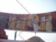
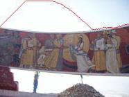
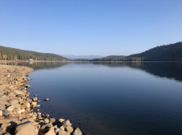
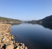
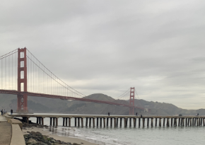
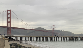
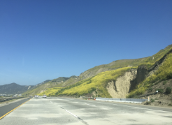
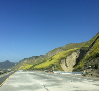
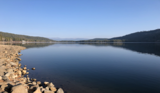
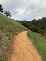
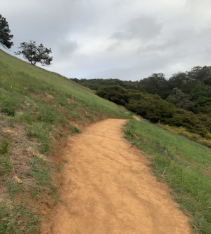
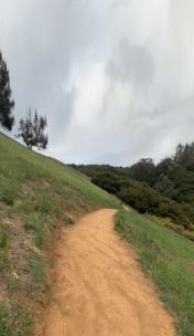
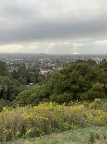
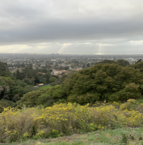
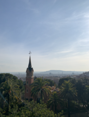
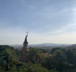
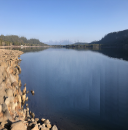
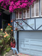
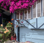
As you can see the seam insertion does pretty well and does not leave any stretching artifacts because we first find the k optimal vertical seams before duplication. However, where the optimal seams are close to highly-structured objects or structured patterns, the seam insertion does not do well because it will distort these highly structured objects and patterns. This can be seen with the tower in Park Guell in Barcelona, Spain and ripples and rocks at Donner Lake. The vertically enlarged image of the lake was more successful than the horizontally enlarged image of the lake.
I learned that content awareness can enhance the resizing of photos rather than simply rescaling. However, it has drawbacks and is definitely not a replacement for choosing the desired aspect ratio at the time of the image being taken. This is because the optimal seams found aren't guaranteed to not interfere with highly structured objects or patterns in the image. This can be seen in my failed results, and it took me time to find images that would be successful for seam carving techniques.
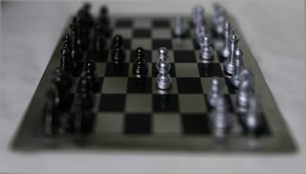
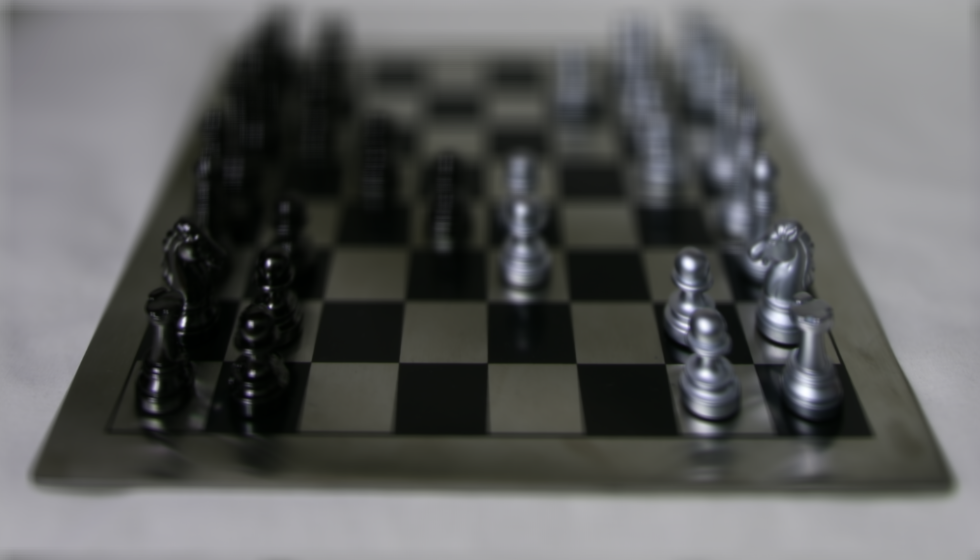
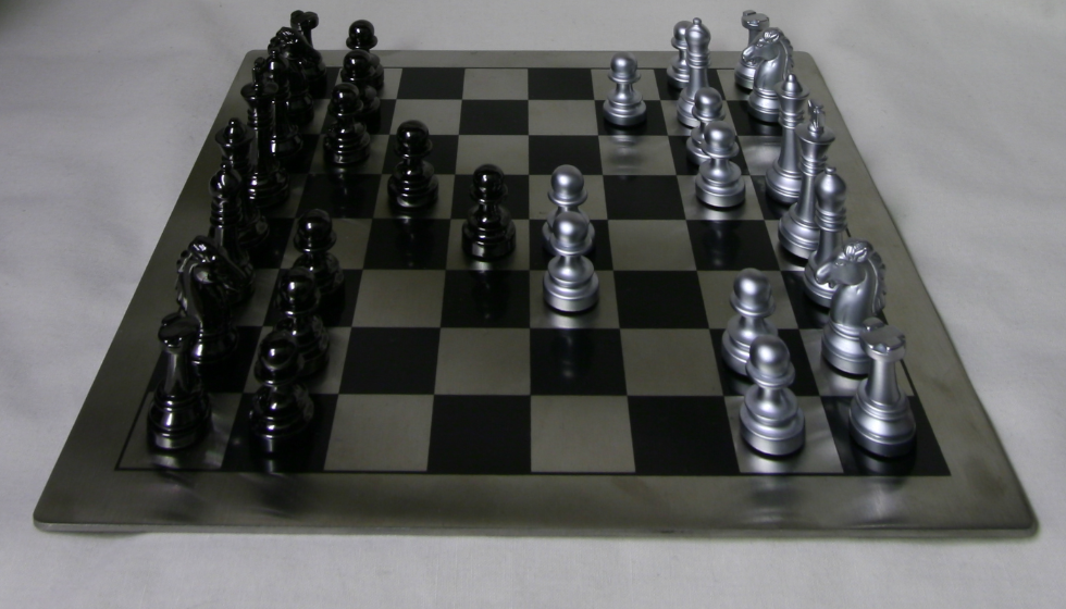
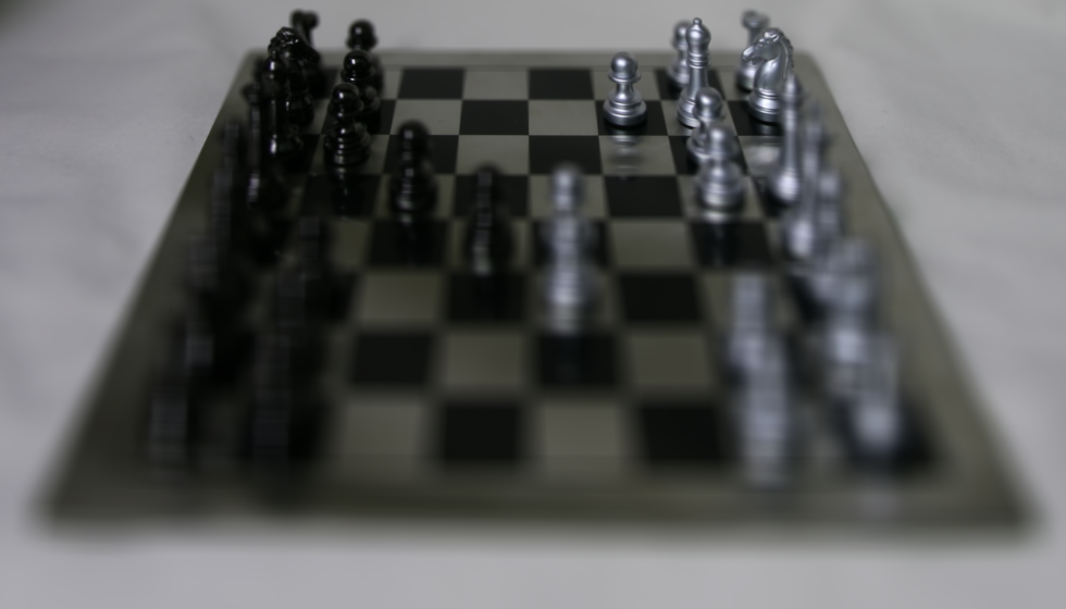
In this project, I reimplemented Depth Refocusing and Aperature Adjustment in the paper, Light Field Photography with a Hand-help Plenoptic Camera by Ren Ng et al. The Stanford Light Field Archive contains a rectified dataset of 289 views of a chess board on a 17 by 17 grid which is what I used.
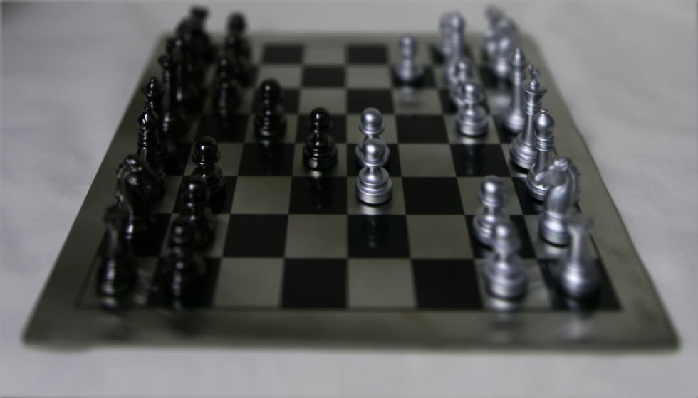
For depth refocusing, objects closer to the camera vary in position accross images more than objects farther from the camera do. Therefore, when you add and average all of the images together, the objects closer to the camera will appear out of focus and the objects farther from the camera will appear in focus.
In order to focus on different parts of the chess board, I shifted each of the 289 view images based on the view's location in the 17 by 17 grid. Then, I chose an amount to scale each shift in order to focus on a specific point. Here are examples of different amounts used to scale the shift. I found these values experimentally.
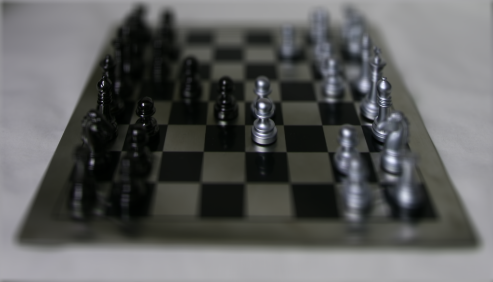
In a camera, the aperature is the hole which light enters a camera and can be manipulated to be large or small. Therefore, averaging all the view images within a large radius from the center of the 17 by 17 grid imitates a camera with large aperature, and averaging within a small radius imitates using a small aperature. This is how I implemented aperature adjustment. I wanted to focus on the center piece of the chessboard in order to see the aperature adjustment more clearly. If the center was in focus, then an image with a large aperature would appear blurry in the back and in the front. I shifted all the images scaled by amount = -1.5 because that is what I found to be the best amount when depth refocusing. Then I only used images in the average if it was inside a specified radius.
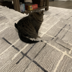
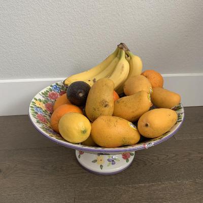
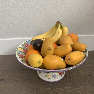
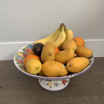
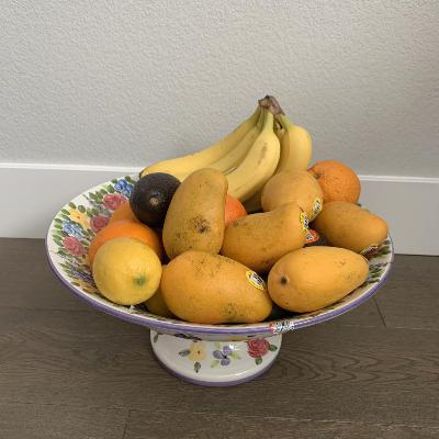
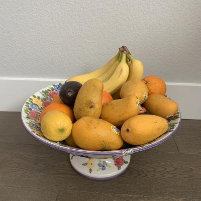
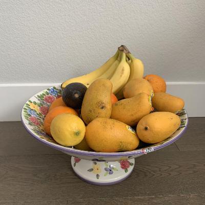
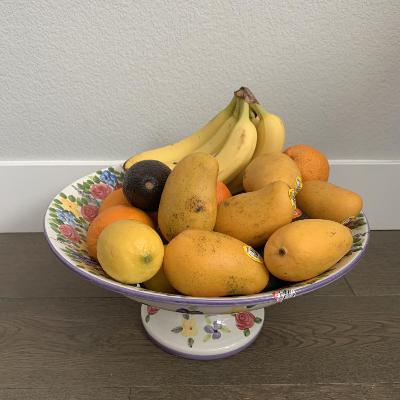
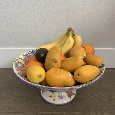
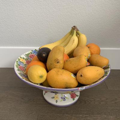
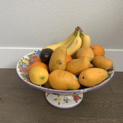
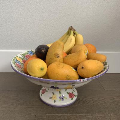
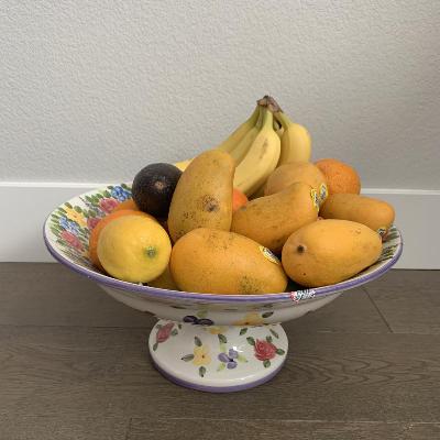
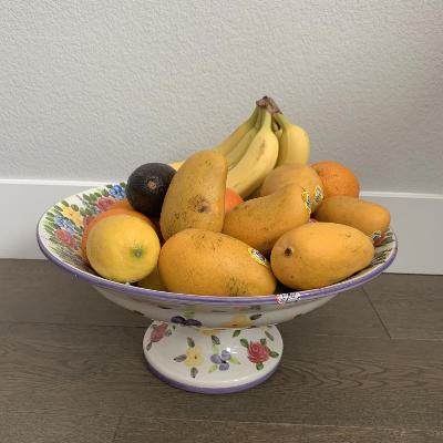
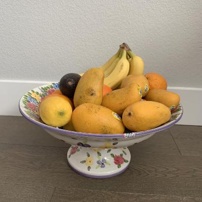
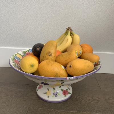
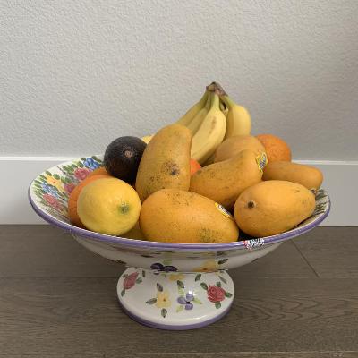
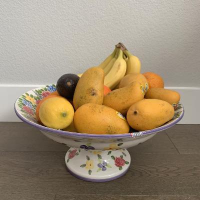
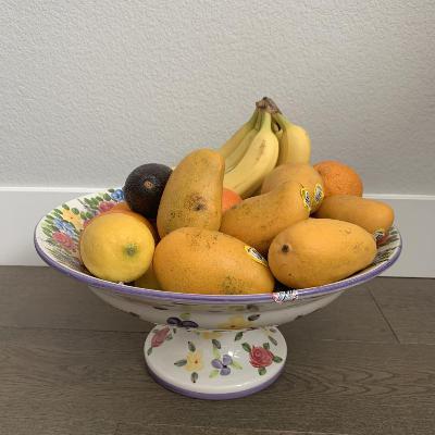
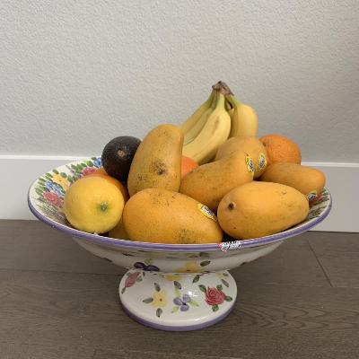
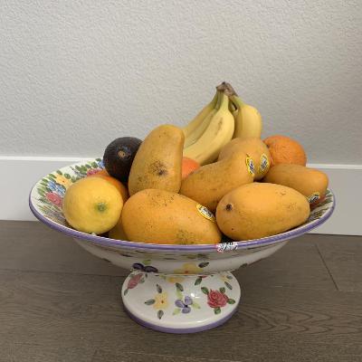
I collected my own data using a 5 by 5 grid. To minimize noise, I tried to make sure the top of the banana was in the same location in each picture. I still expected there to be imperfections due to inaccurate locations, rotations in my image-taking, distracting background, and non-correspondence between the 25 images. Here are my images in the 5 x 5 grid.
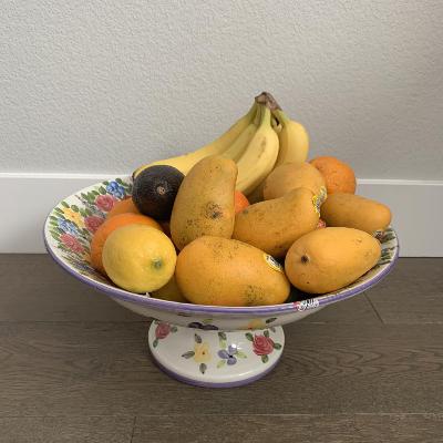
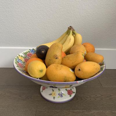

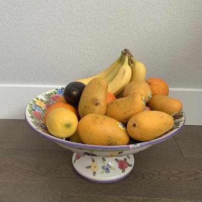
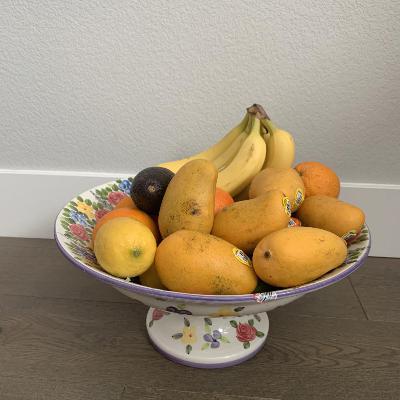
For depth refocusing, the amount I scaled each shift was range(0, -10, -1) For aperature adjustment, the amount I scaled the shift for all images was 0 and the radii were range(0, 4, .4)
As you can see, it did not work as well as the chess image dataset from The Stanford Light Field Archive due to the inaccurate position of my camera taking the pictures and the non-correspondence. In the depth refocusing, the bananas which are the farther away objects do get more and more unfocused. However, they never started out in focus because of the innacuracies of the image-taking. In the aperature adjustment,you can see the wall behind the bananas and fruit in front do become blurrier as the aperature gets larger. However, due to the inaccuracies from image-taking, averages using a small radius are very noisy and contain a lot of ghosting.
I gained a deeper understanding of depth and aperature while working on this project. I learned how taking multiple grid-structured images could recreate a camera effect and do powerful things.