CS194-26 Final Project
Gradient Domain Editing and HDR Image Toning
Gradient Domain Editing
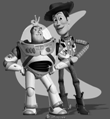
The gradient domain algorithm can be principally viewed as a least squares, optimization problem. The unknowns are the pixels in the region to be replaced, constrained by the existing gradients in the original source image, as well as a smooth transition at the seam. Solving an overdetermined system of equations with least squares implicitly assumes smooth solutions, and may not always be the best solution, especially along the seam cuts, and can blend / interpolate with strange artifacts, so a uniform region cut is desirable. The below examples also include a choice to constrain over the maximum gradient between the source and target image, which, in general, produces desirable results (especially to enable smooth color transitions for two vastly different images), but as shown may interrupt smooth regions of the source image.
Toy problem.
Copied image with least squares, save the borders of the image, still black.
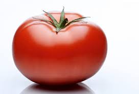
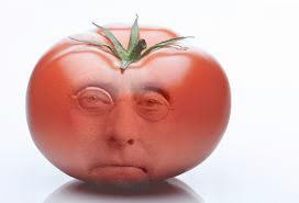
tomato
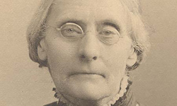
woman
Final morph, nonmax gradient.
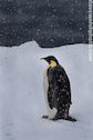
penguin
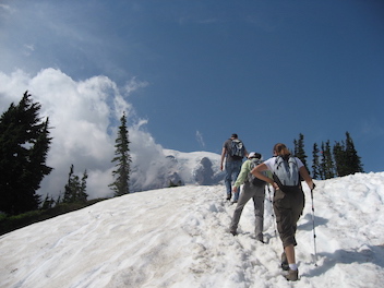
hikers
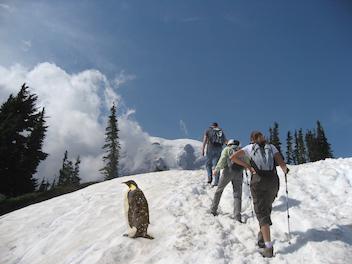
Final morph, nonmax gradient.
penguin
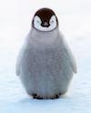
chick
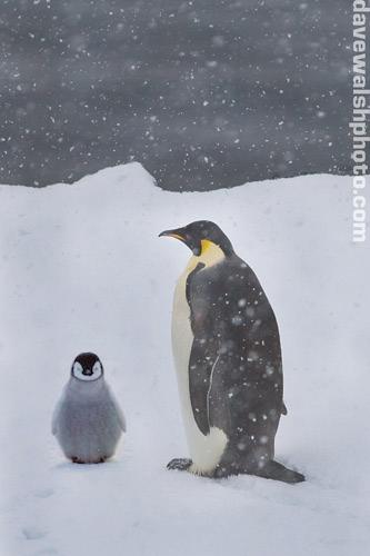
Final morph, nonmax gradient.
Bells and Whistles: Using Max Gradient
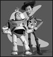
Final morph, max gradient. Notice the image is less grey.
Final morph, max gradient. Snow retains its dunes and texture, but interrupts with the penguin's belly.
Final morph, nonmax gradient.
HDR Imaging
Irradiance transform
The first part of the algorithm, identifying the inverse transform between received pixel intensity and linear radiant intensity, is a least squares problem, setting the unknowns being the radiant intensities at each pixel position in the stack, and the transform function for each pixel value (0-255). The least squares function, using sparse matrices, is relatively simple. Irradiance is visualized as a global tone mapping with a simple log applied. For the least squares, smoothing penalty functions are also added, added to a heavy penalty to make sure the g function is normalized to 0 at pixel value 127. This was to ensure normalized response between color channels. Even then, a bit of color exaggeration exists, due to slight offsets between channels. Only ~100-150 pixel locations per exposure level are really necessary - beyond such a number provides no better accuracy, at least at the level of human perception.
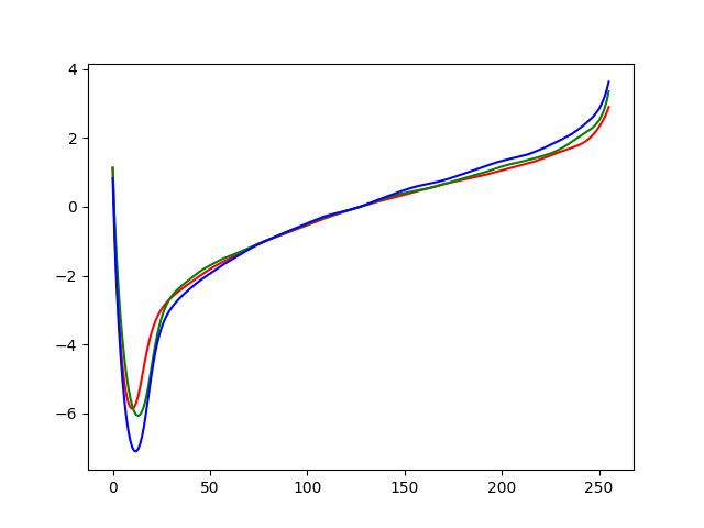
Transfer function for the chapel. 0 values had a strange artifact due to how z values were randomly sampled. Z-values were uniformly queried on the median image - but the median image in this case lacked pixel values between 0 and 21. Nevertheless, since the weight of low intensity pixels is small, this had negligible effect on the ultimate result.
Log response of radiance map.
Local Tone Mapping
A lot of grief went into this function. The principal idea, from Durand, involves only a reduction in the blurred log domain of the radiance map, compressing it into 4-5 levels, and then re-adding the difference, detailed levels. Using a bilateral filter in principal blurs the image while locally preserving edges, inversely weighted by the intensity difference. This "in principle" fact would not hold, however - the difference layer would often had radiances far exceeding the (-inf, 0) log exposure limit, thus far overriding the base effect. My fix, following, involves also contrast-reduction in the difference layer, followed by adhoc contrast and saturation adjustment using 1)White balancing, 2) contrast response function on pixels, and 3) saturation increase by adding to the S channel in HSV space. Also, outliers were removed by histogram culling, removing any colors that had fewer than some 0.05% or custom threshold of all pixels. Finally, gamma correction was applied.
Blurred image after bilateral filtering.
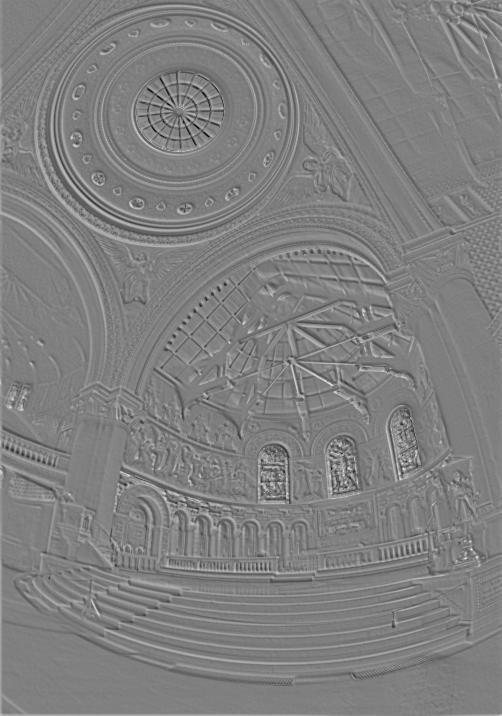
Difference image after filtering.
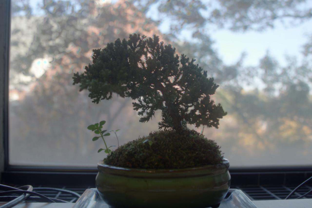
Global tone mapping for bonsai.
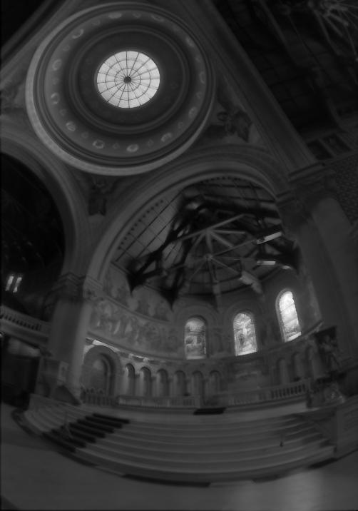
Global tone mapping for chapel.
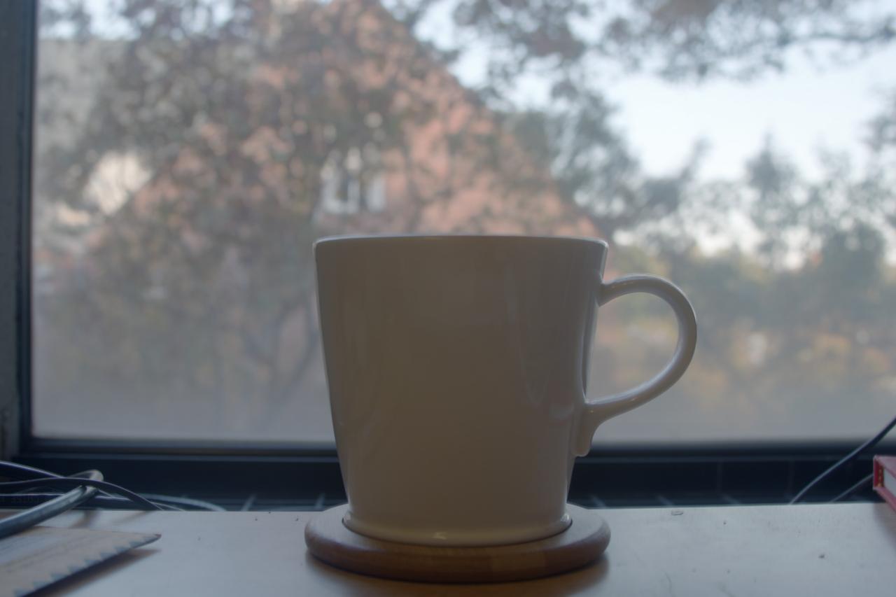
Global tone mapping for mug.
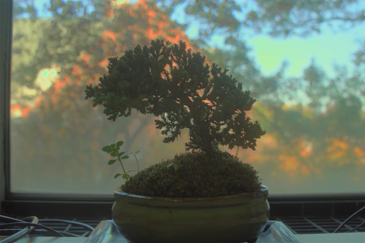
Local tone mapping for bonsai. Notice the richer window colors.
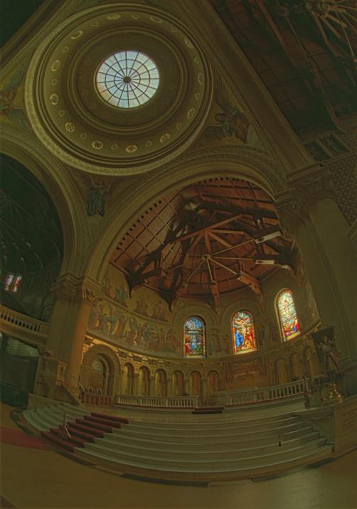
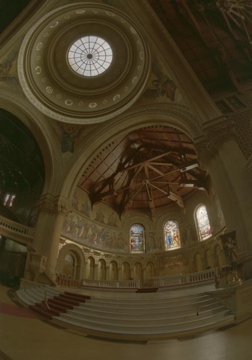
Local tone mapping for chapel.
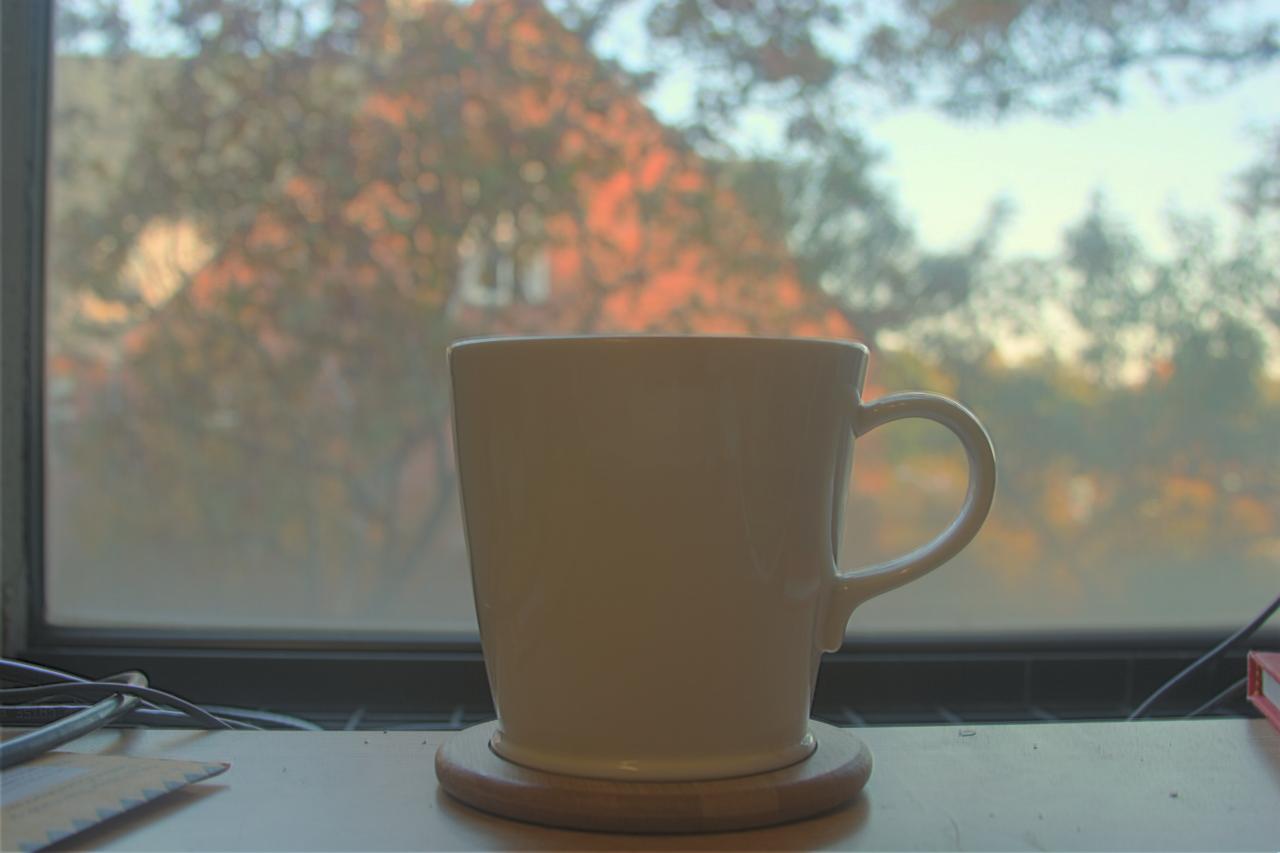
Local tone mapping for mug.
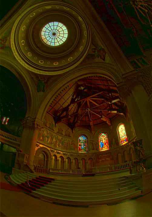
Local tone mapping for chapel with basic color correction.
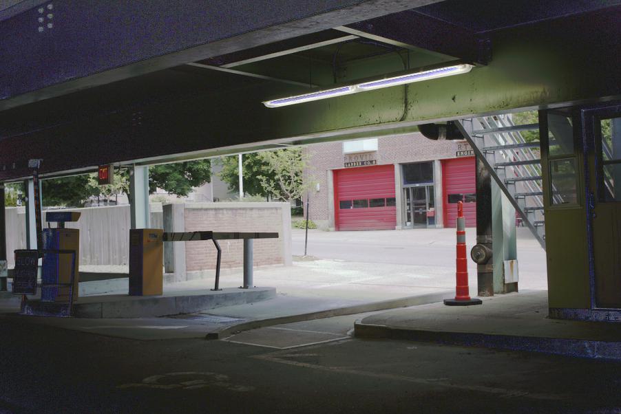
Garage.
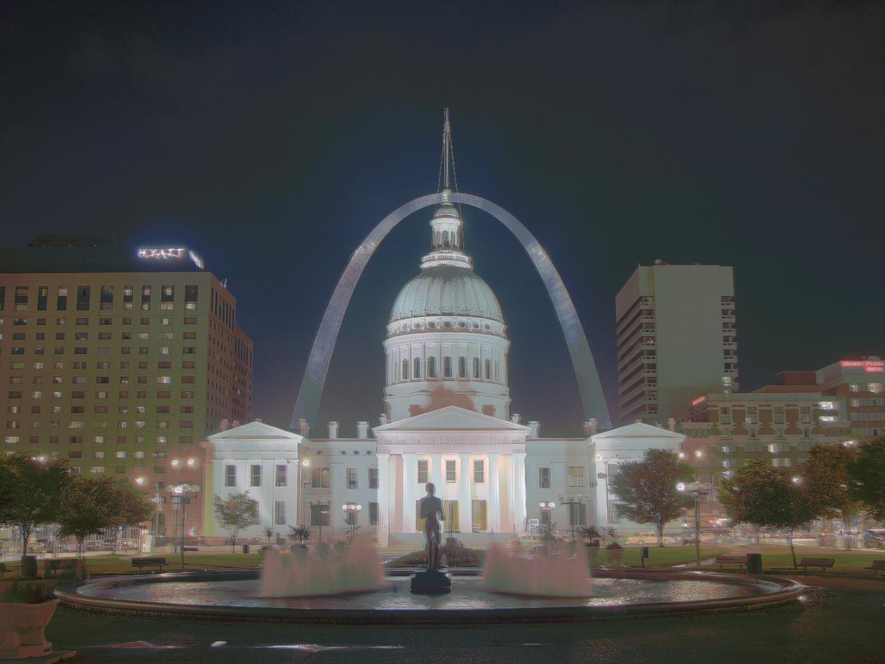
arch.