Project 1: Seam Carving
Overview:
Seam carving is a way by which we can shrink an image, either horizontally or vertically, by removing the seam of
lowest importance in an image. The general overview of the algorithm is for each seam that we want to remove, compute
the importance of every pixel in the image using an energy function, and then using a dynamic programming algorithm
given in the provided paper, find the lowest-importance seam in the image. We can then remove the seam in the image
to resize the image by that one column or row!
Energy Map:
The first step to finding the current minimum seam of an image is to use an energy function to compute the importance of
every pixel in the image. Following the procedure in the provided paper, what I did was take the gradient with respect to x (Dx)
and the gradient with respect to y (Dy) for each color channel of the image. Then, I computed the SSD of Dx and Dy, before averaging
the results of each color channel to get a final energy map. Below are two input images, as well as their corresponding energy maps:
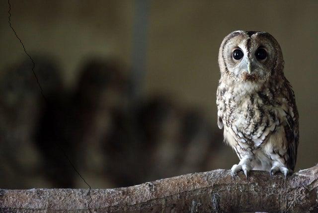
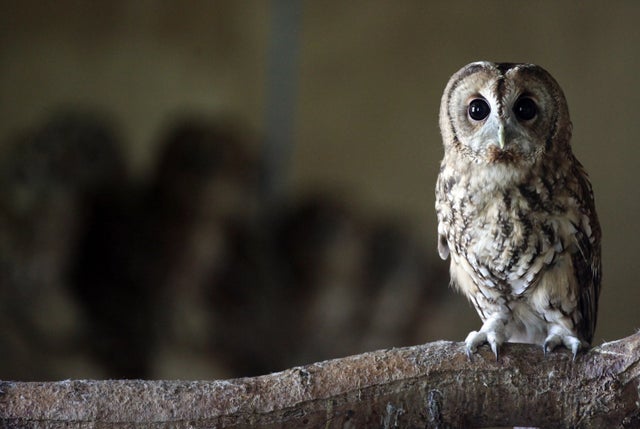 Owl
Owl
|
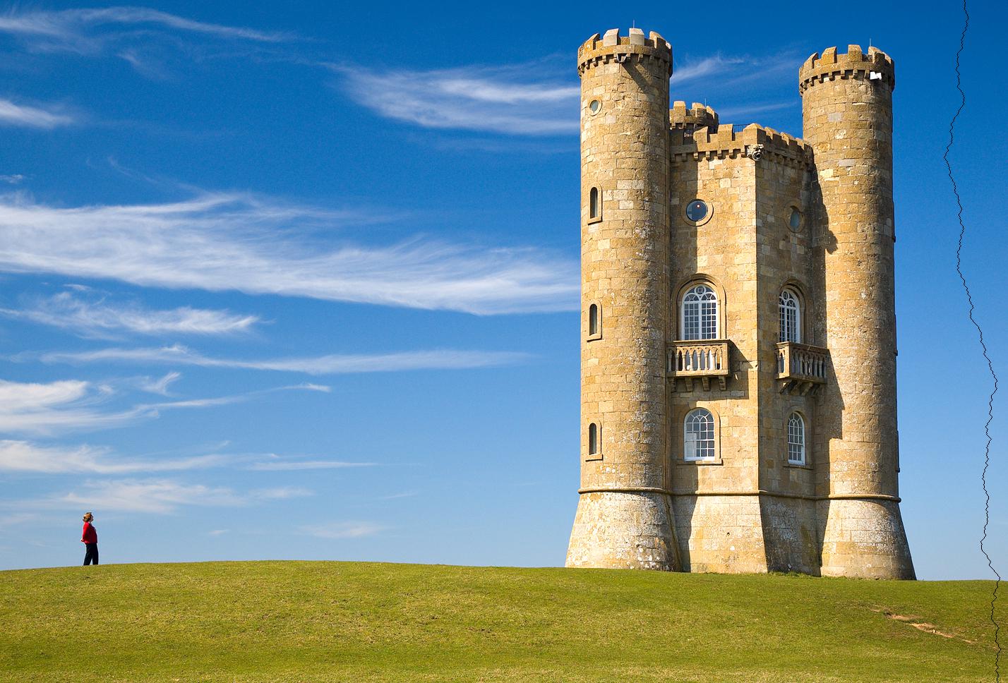
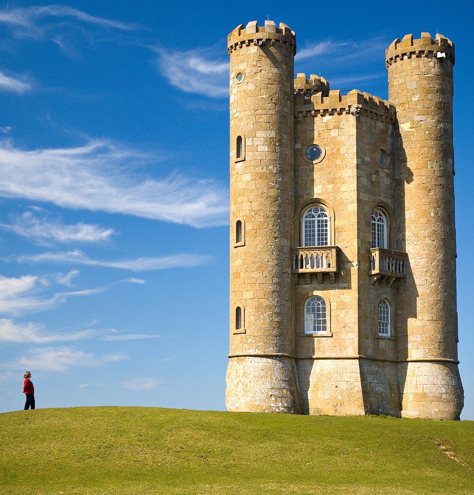
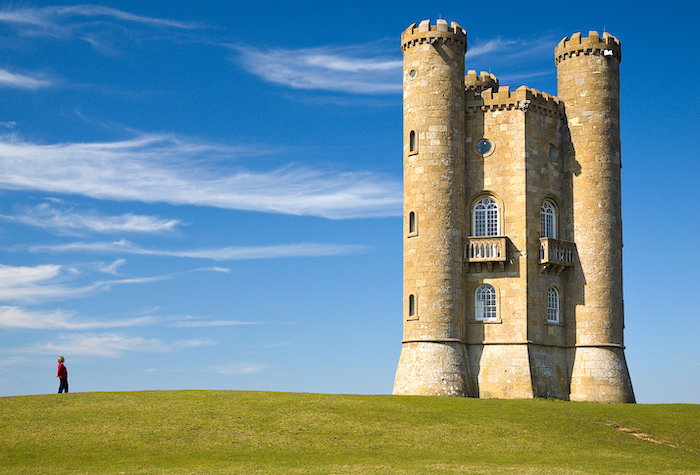 Tower
Tower
|
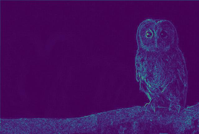 Owl: Energy Map
|
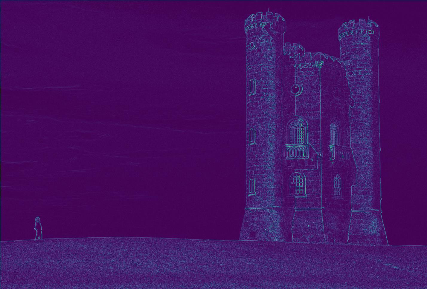 Tower: Energy Map
|
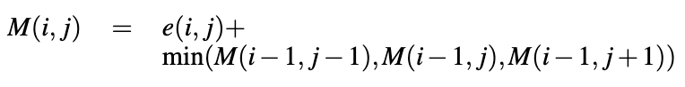
Minimum Seam:
Now to compute the minimum seam using the energy map, what I had to do was initialize a numpy array
called minimum_energy, then update values of the next row using the following dynamic programming
recurrence relation:
I also initialize a prev array that keeps track of the index of the previous element as it updates the
values downward. Upon going through the entire image and computing the values from the algorithm, I then
find the index of the smallest energy value in the final row, and use the prev array to iterate backwards
between the rows to create a mask for the image, where values along the minimum energy seam are zeroed out. Below are the
results of the same images as before, where the current minimum seam is zeroed out. Notice the seam tends to go through
areas of the image which have relatively little importance and change throughout:
 Owl With Seam (Black line on left)
|
 Tower With Seam (Black line on right)
|
Lastly, I used this computed mask on my image to effectively downsize the image, removing the
pixels along the seam! Doing this multiple times results in appropriate downsizing of the image,
where we always remove seams of minimum importance to create a very natural looking shrinking process.
Horizontal Carving:
The previously described process, removing seams that are vertical along the image, is known as horizontal
carving. I managed to do this for multiple images, often choosing arbitrary downsizes to test the limits of the
resizing that would leave minimal artifacts. Below are some finalized results, with the original image on the left,
and resized image on the right:
|
Owl: Original
|
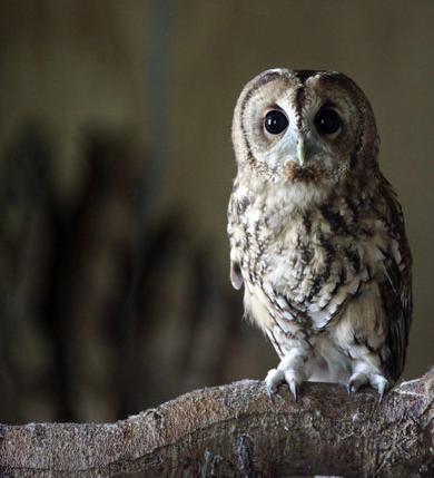 Owl: Horizontal Carving (250)
|
|
Tower: Original
|
 Tower: Horizontal Carving (500)
|
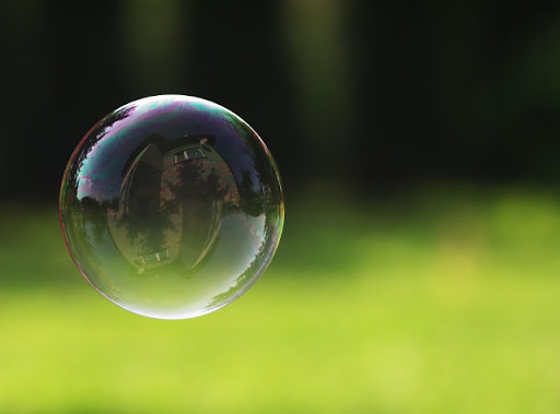 Bubble: Original
|
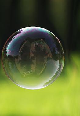 Bubble: Horizontal Carving (250)
|
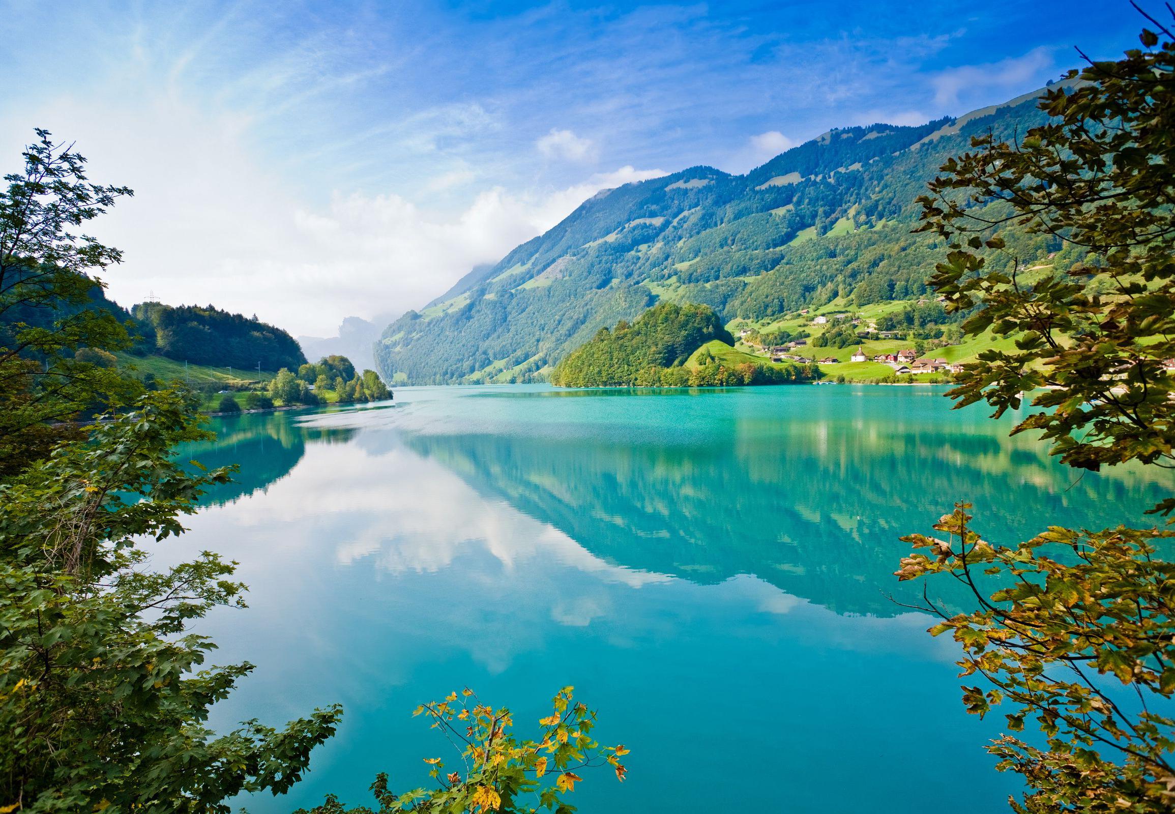
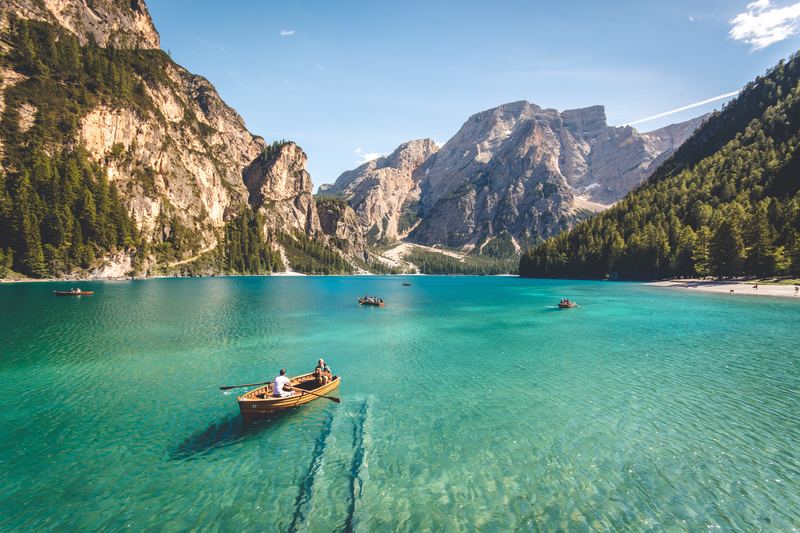 Lake: Original
|
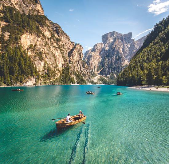 Lake: Horizontal Carving (250)
|
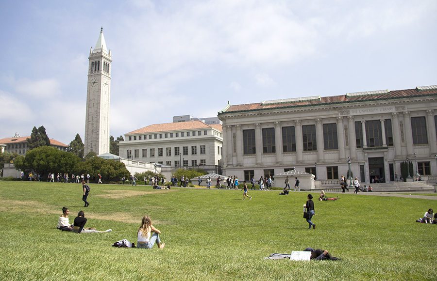 Berkeley: Original
|
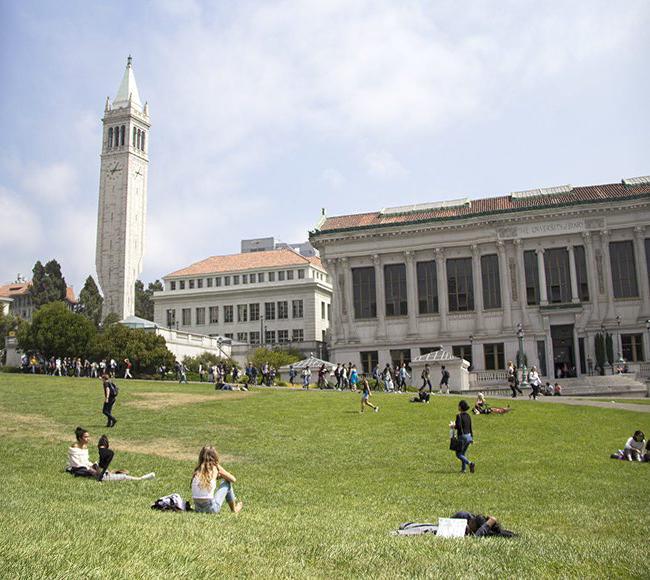 Berkeley: Horizontal Carving (250)
|
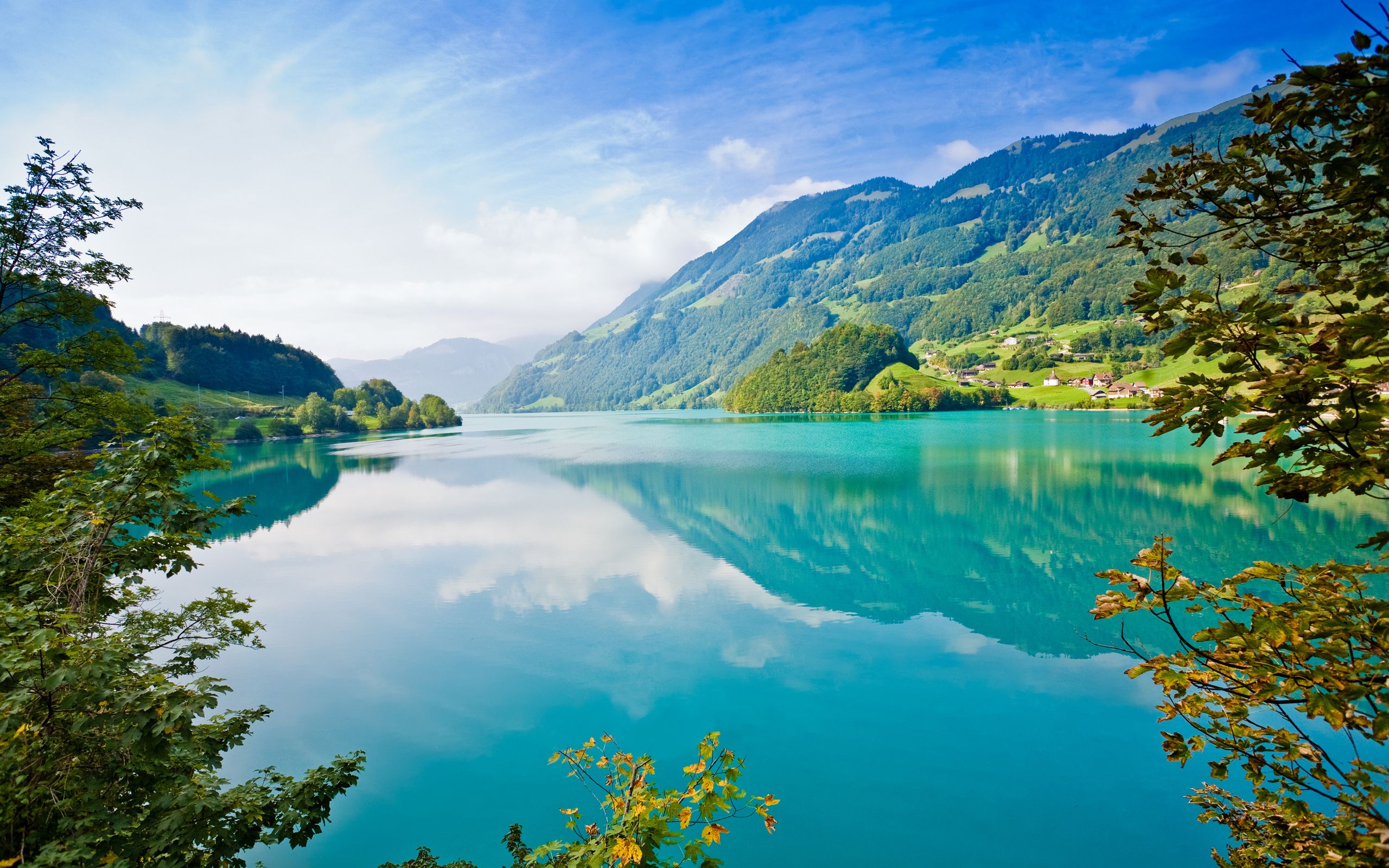 Mountains: Original
|
 Mountains: Horizontal Carving (250)
|
Vertical Carving:
Similarly to horizontal carving, instead of finding the minimum seam vertically, I could instead find the minimum seam
horizontally, and remove that, innately removing a row of the image and shrinking it vertically. Doing so is called
vertical carving, and allows us to resize our images in a slightly different manner. The only difference in implementation
of vertical carving compared to horizontal carving is that before computing the energy map and finding the minimum seam vertically,
we can just transpose the image first. That way, the minimum column-wise seam is actually the minimum row-wise seam. The procedure
follows from this in the same way, where at the very end, I just transpose the image back to get the vertically carved result. Below are
some results of vertical carving:
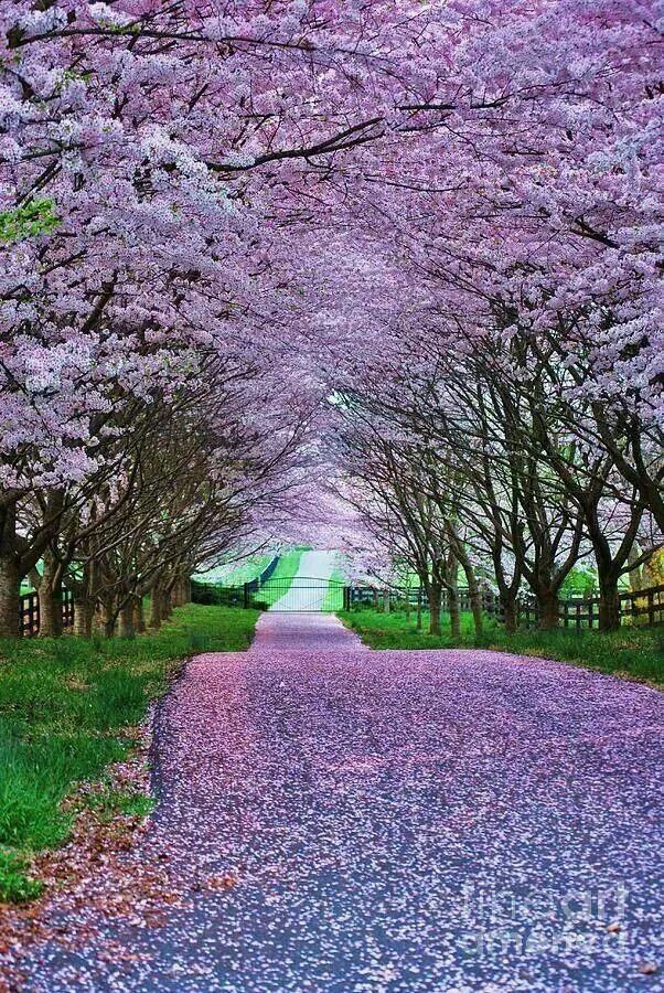 Flowers: Original
|
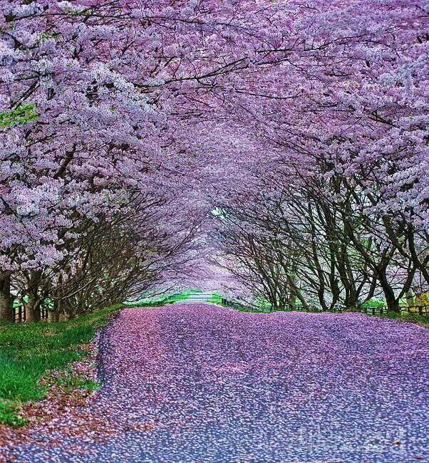 Flowers: Vertically Carved (250)
|
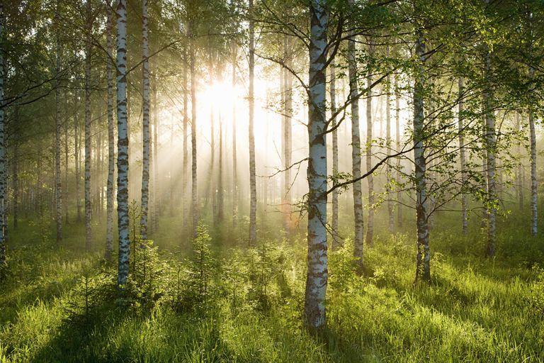 Forest: Original
|
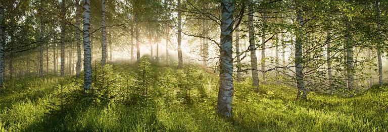 Forest: Vertically Carved (250)
|
Failure Cases:
Although seam carving is very effective at naturally shrinking scenes, it still has its limits.
When trying to downsize too much, eventually even the minimum seam will be of relatively high
importance, and it will fail to preserve many of the prominent features in the image, resulting
in a lot of aliasing. For example, below are some results of the Berkeley image horizontally carved
to a larger degree. Notice how as we carve more and more, eventually the structure of the straight lines
in the image begins to give way, as the buildings and people become curved:
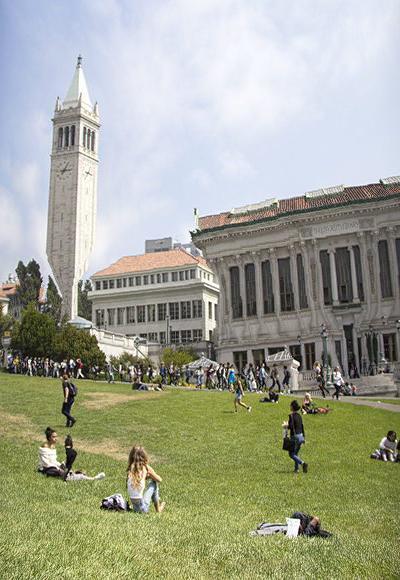 Berkeley: Horizontally Carved (500)
|
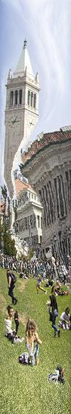 Berkeley: Horizontally Carved (800)
|
Additionally, seam carving has relatively poor results when needing to preserve the ratio between
features within the image, such as maintaining the shape and structure of faces. Below is one such
example of this failure, showing how Pikachu gets hopelessly distorted even with a relatively small
horizontal carving:
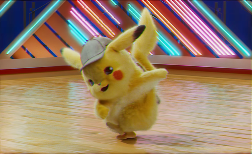 Pikachu: Original
|
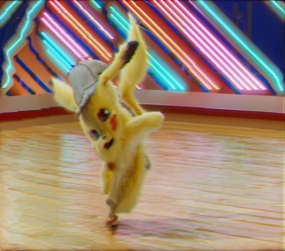 Pikachu: Horizontally Carved (250)
|
Bells and Whistles: Diagonal Resizing
I implemented optimal diagonal resizing for images using my previous functions, essentially resizing both vertically and
horizontally in the optimal order, by always taking the minimum of both the minimum horizontal seam and the minimum
vertical seam. As a result, I was able to effectively achieve a given height and width by inputting the appropriate
dimensions to be shaved off from either axis. Below are some results of the diagonal resizing, using some of my previous
images:
|
Tower: Original
|
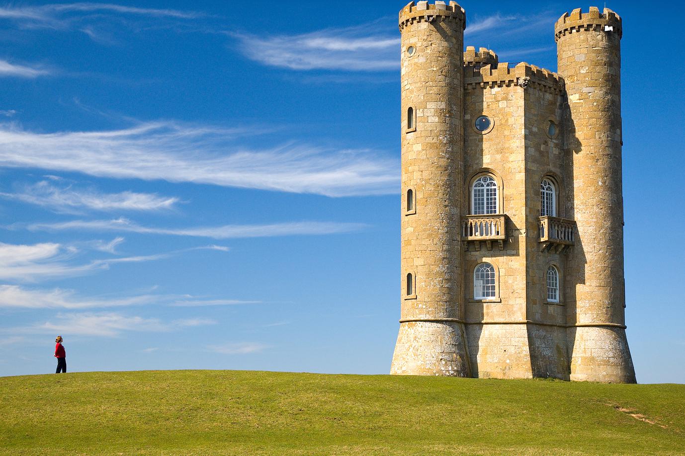 Tower: Diagonally Resized (50, 50)
|
|
Lake: Original
|
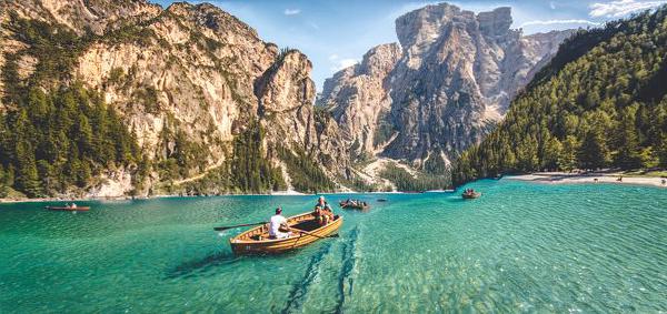 Lake: Diagonally Resized (200, 250)
|
What I learned
From this part of the final project, the most important thing I learned was how simple it is to resize images elegantly, and how
effective the results of this can be. Relatively basic computations, such as SSD for an energy map and a basic dynamic programming
algorithm can lead to such impressive results, and its really cool how this can be done in real time to intelligently resize images!
Project 2: Lightfield Camera
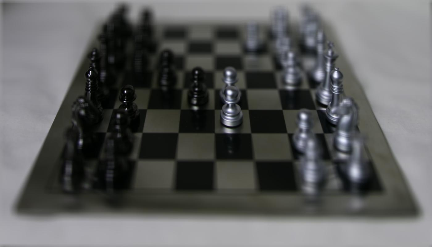
Overview:
With multiple images taken over a regularly spaced grid, I was able to replicate the effects of depth refocusing and changing
aperture size by aliging and averaging various images appropriately. Using sample data from the Stanford Light Field Archive, I observed
how different methods of averaging these pictures taken in a grid could result in different visual effects. Note that I used the
chessboard dataset from the Stanford Light Field Archive to display theses effects.
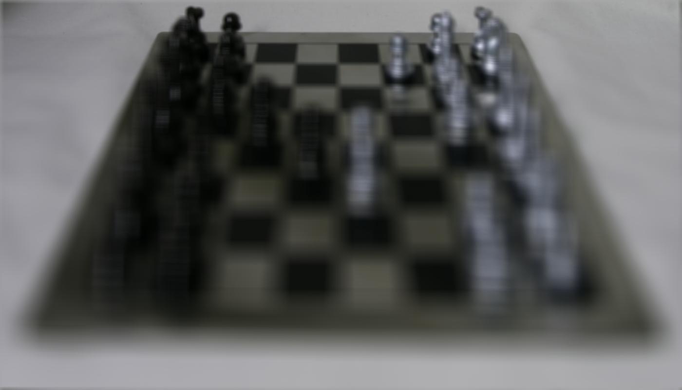
Depth Refocusing
In order to implement depth refocusing, I first took the center light field image at index (8,8), using that as a reference point. Then,
for every other image in the dataset, I shifted each image by (u_shift, v_shift) = constant * (u_curr - u_center, v_center - v_curr), where
the constant is chosen as input to decide how far away the image should focus. These shifted images are all then averaged together along
with the center image to produce a result that is focused on a specific area!
Experimenting with various constant values to determine where the focus point was, I found that lower constant values, up to around
-0.6, result in focusing closer to the camera, whereas higher constant values, up to around 0.1, resulted in focusing further away.
Too much outside of this range resulted in blurry images overall, as the shift was too big and the focus point would not be visible
within the image dimensions. Below are examples of the chessboard focusing at different points, with the corresponding constant (c)
values, as well as a gif of 50 frames showing a gradual change in (c) value from -0.5 to 0.1:
 C = -0.6
|
 C = -0.5
|
 C = -0.4
|
 C = -0.3
|
 C = -0.2
|
 C = -0.1
|
 C = 0.0
|
 C = 0.1
|
 C = 0.2
|
 C = 0.3
|
 GIF: C = [-0.5, 0.1]
|
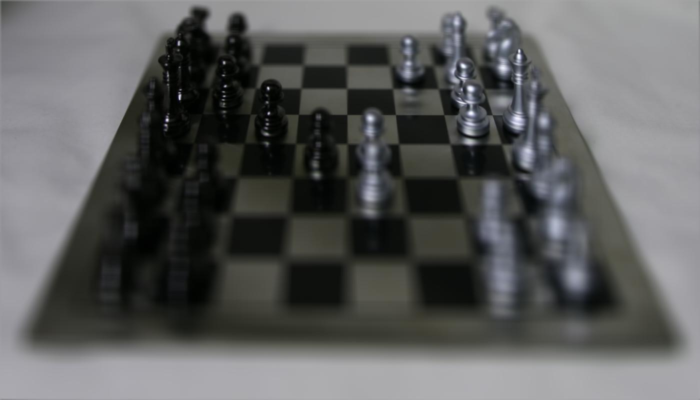
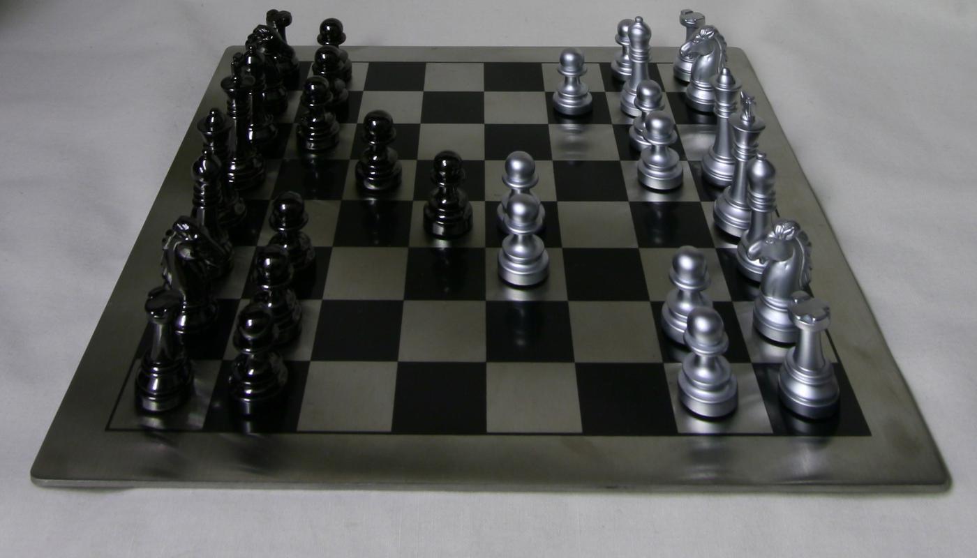
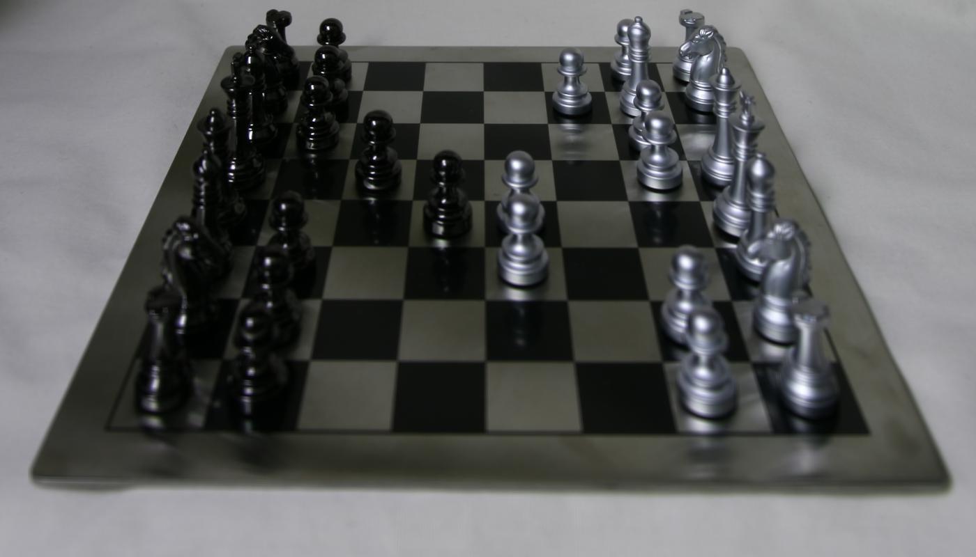
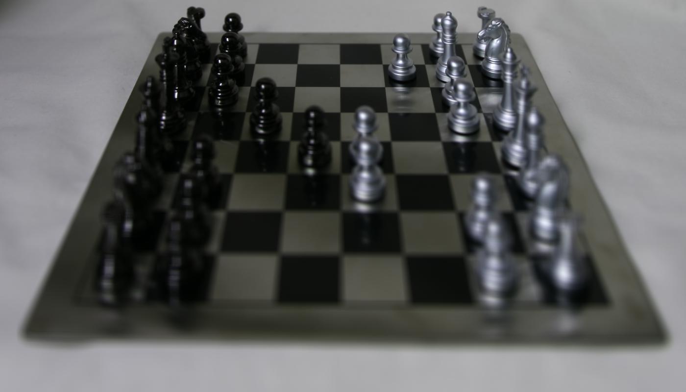
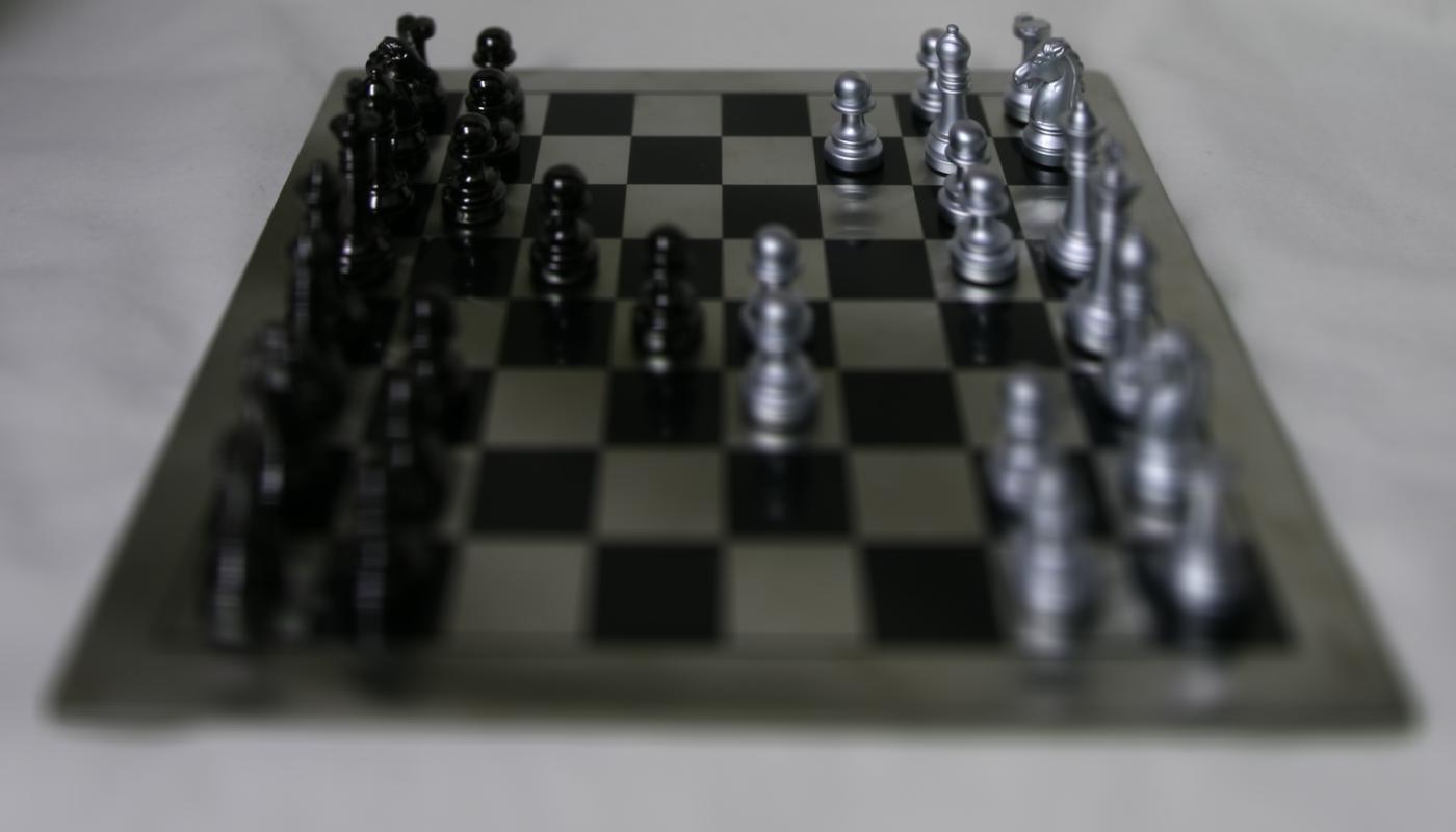
Aperture Adjustment
In order to simulate aperture adjustment using the same dataset, using the same (8,8) image as my central reference point,
what I did was to only average other images together of a specific radius away from the center, choosing that radius value
based on what size of an aperture I wanted to simulate. The larger of a radius chosen, the more images are averaged together,
and the larger of an aperture size is simulated. Similarly, the less images that are averaged together results in a smaller
aperture size. Below are results of simulating changes in aperture size, labelled by the radius chosen, as well as a gif
representing changes in aperture size. Notice how the focal point always remains the back of the chessboard, but the changing
aperture size affects how the rest is in focus:
 Radius = 0
|
 Radius = 1
|
 Radius = 2
|
 Radius = 3
|
 Radius = 4
|
 Radius = 5
|
 Radius = 6
|
 Radius = 7
|
 Radius = 8
|
 GIF: [1, 8]
|
What I learned
The coolest thing here was how everything was really simple to implement, mostly resulting in
simple shifting and averaging techniques, even going back to something like the first project! I really
liked seeing how we could simulate these cool image effects manually, and how everything nicely came
together. I especially liked how cool depth refocusing looks within images, and its really amazing that
a simple algorithm like this can allows something that looks really complex to work! Overall, this class
was really great, and I definitely learned a lot from all the projects and the experience!