In this project, we implemented the seam carving algorithm outlined by Avidan and Shamir in their SIGGRAPH paper. Seam carving allows for content aware resizing of images. Rather than scaling the entire image by a certain factor when decreasing its width or height, seam carving chooses specific seams that are considered the "least important" in the image and removes them. A seam is a line of continuous pixels stretching from either the top to the bottom (vertical seam) or left to right (horizontal seam) with one pixel from each row or column.

In many photos, using this technique results in a large portion of the background being removed, but with objects in the foreground maintaining their shape and prominence in the image, thereby making the resizing process "content aware".

The energy function is used to determine which pixels in the image are the least important and should be removed first. For this project, I used the basic energy function proposed by the paper: E(I) = |d/dx(I)| + |d/dy(I)|. At each pixel, this energy function computes the sum of the absolute values of the change in X and the change in Y of the pixel values by retrieving the pixel values of its neighboring pixels in the vertical and horizontal directions.

Next, we implemented a dynamic programming algorithm to identify the lowest energy seam to remove. In this overview, I'll be discussing the approach for vertical seams, though a symmetrical approach can be applied to horizontal seams. We begin by allocating some memory to store the cumulative minimum energy seam at each pixel in the NxM image. The minimum energy for the top pixels is initialized first, simply by computing the energy at each of those top pixels. Then, for Rows 2 through N, we use the following step to compute its cumulative minimum energy from the top of the image up until the current pixel's row:

M(i,j) = E(i,j) + min( M(i-1, j-1), M(i-1, j), M(i+1, j+1) )

This step computes a pixel's minimum cumulative energy by adding its energy to the minimum cumulative energy of the candidate pixels above it. Because the seam must be a continuous line, the only candidate pixels in the row above it are the one whose x-value is at most 1 value away.

Once we've completed this process for Row N, we can conclude that the pixel with the lowest cumulative minimum energy in that row is part of the lowest energy seam in the image. We then backtrack upwards to determine the full seam, and can correspondingly remove that seam of pixels from the image. We repeat this process until the image has shrunk to the desired size.

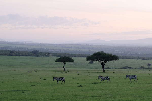
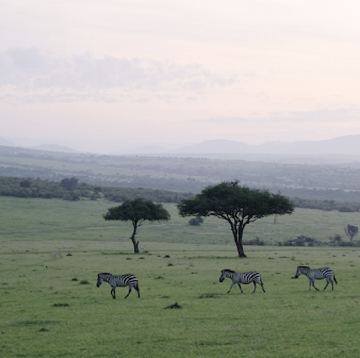
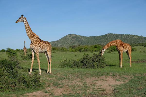
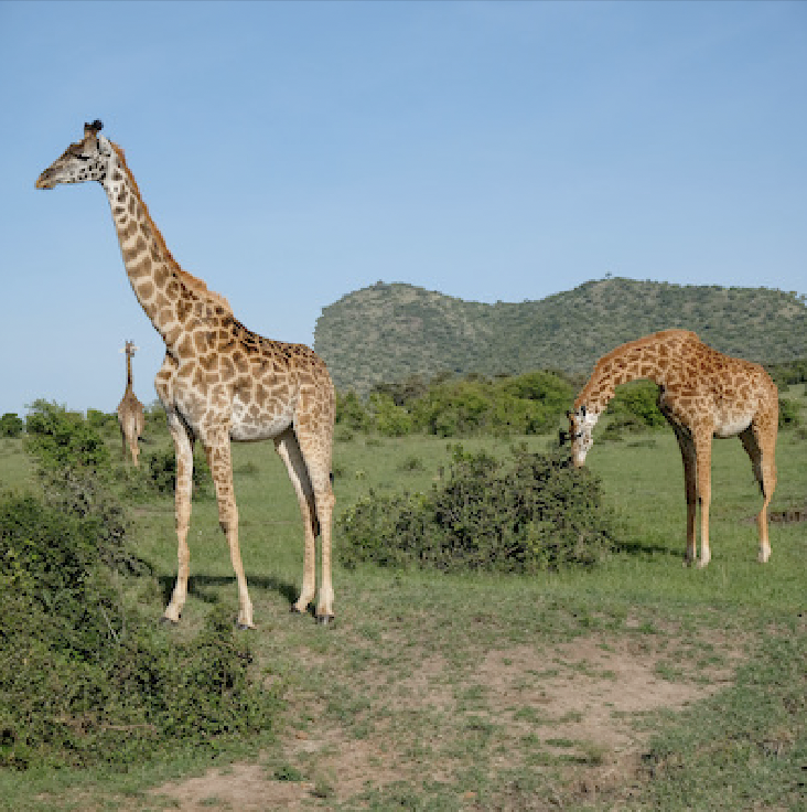
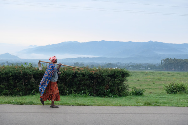
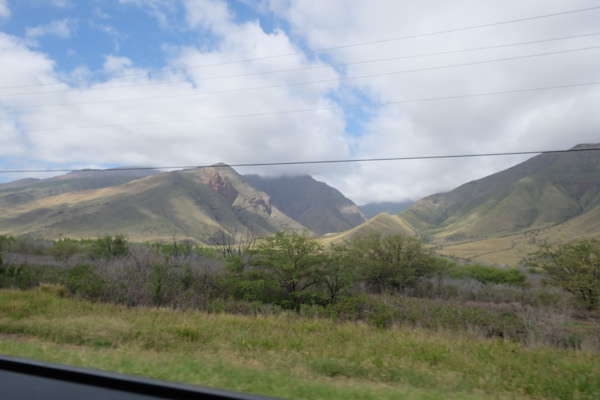
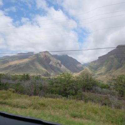
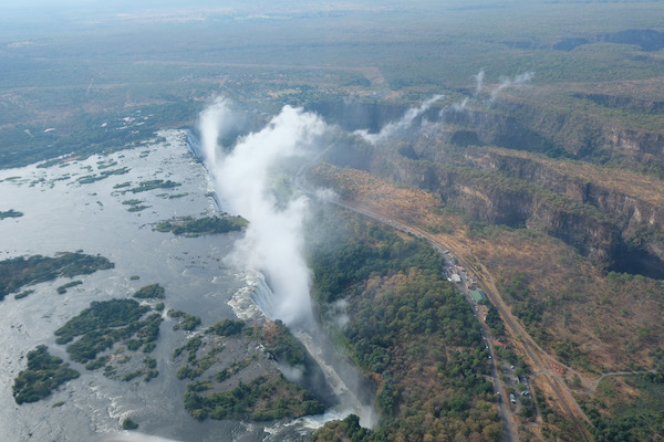
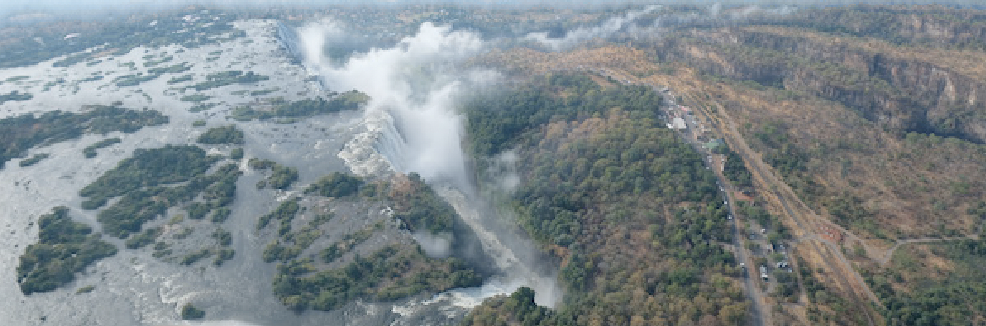
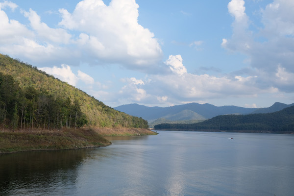
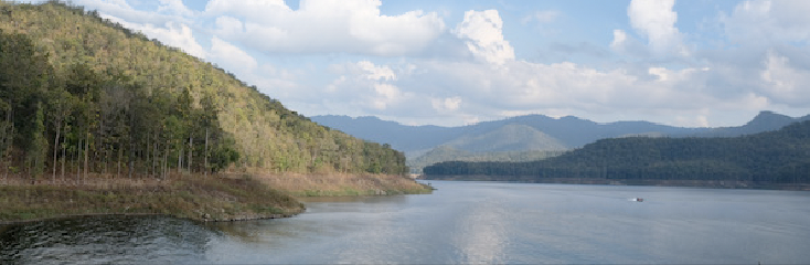
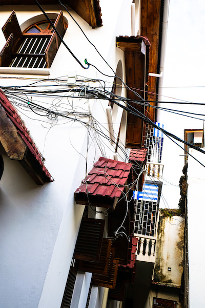
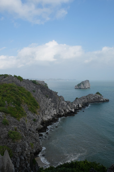
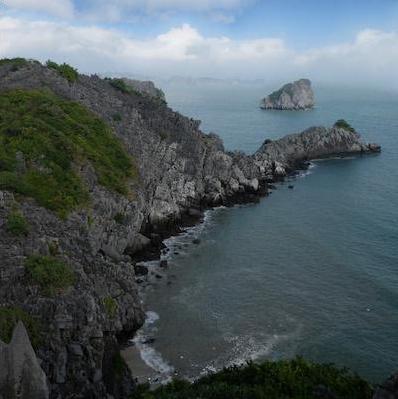
Below are some examples of horizontal carving, where we removed vertical seams and decreased each image's width by 200 pixels!

Below are some examples of vertical carving, where we removed horizontal seams and decreased each image's height by 200 pixels!

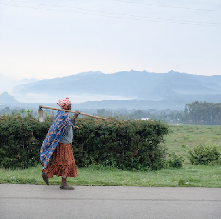
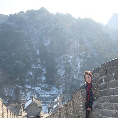
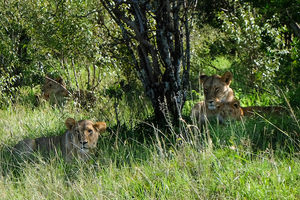
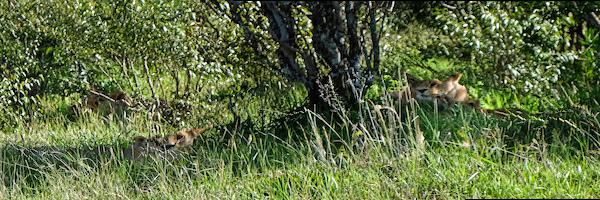
Below are some failure cases of my algorithm. In "Great Wall" and "Aloha", we see that the algorithm does not do particularly well with faces. Face structure is important in making the image look "natural", but unfortunately the seam carving algorithm does not account for things like the geometry of certain shapes and instead only looks at the gradients between pixels. This is why the faces in "Aloha" look particularly distorted because although the pixels were deemed "least important" before removal, they ended up warping the face structure and shape of the people pictured. In "Great Wall", the image has a lot of complex textures in the background which additionally end up being determined as "important" by our energy function because those small changes resulting from the textured background are considered, whereas the clothing that I am wearing is much less textured and therefore is counted as "less important". Furthermore in "Lions In Wait", the image is pretty dark around the lions, so the energy function has more of a difficult time distinguishing between those pixels. Similar to the other images, this image also struggles with maintaining the face structure of the lions.

In this project, we used multiple images of the same scene captured over a regularly spaced grid to produce the effects of refocusing the scene at different depths and adjusting the aperture size. As explained by Ren Ng's paper on light field photography, capturing these images over a plane orthogonal to the optical axis allows us to use shifting and averaging operations to create these effects.

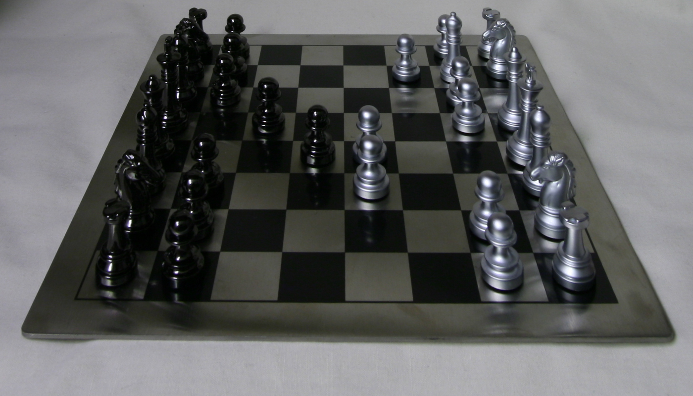
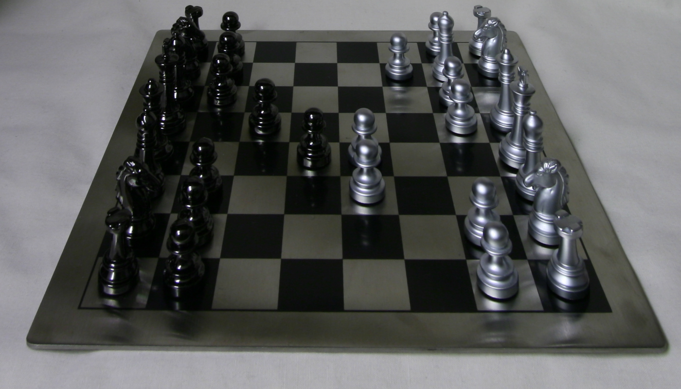
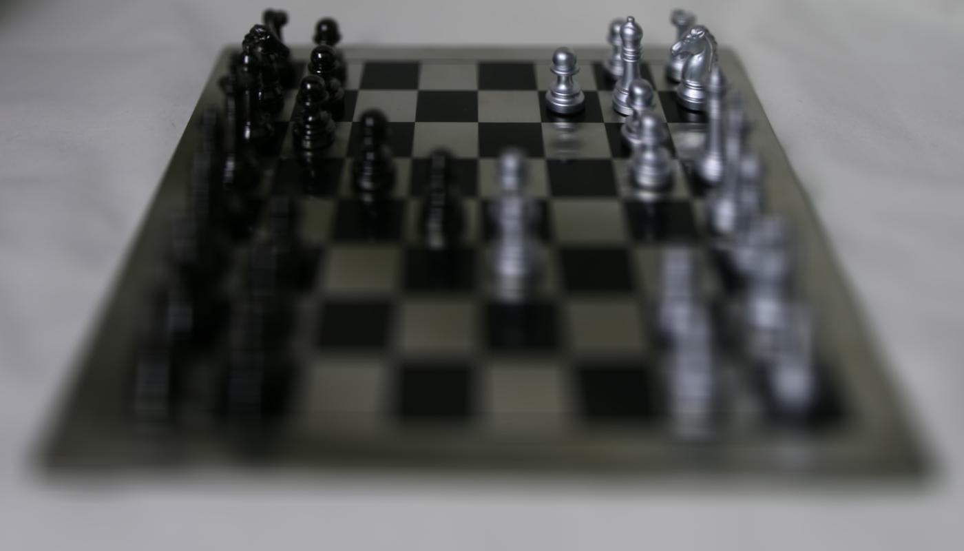
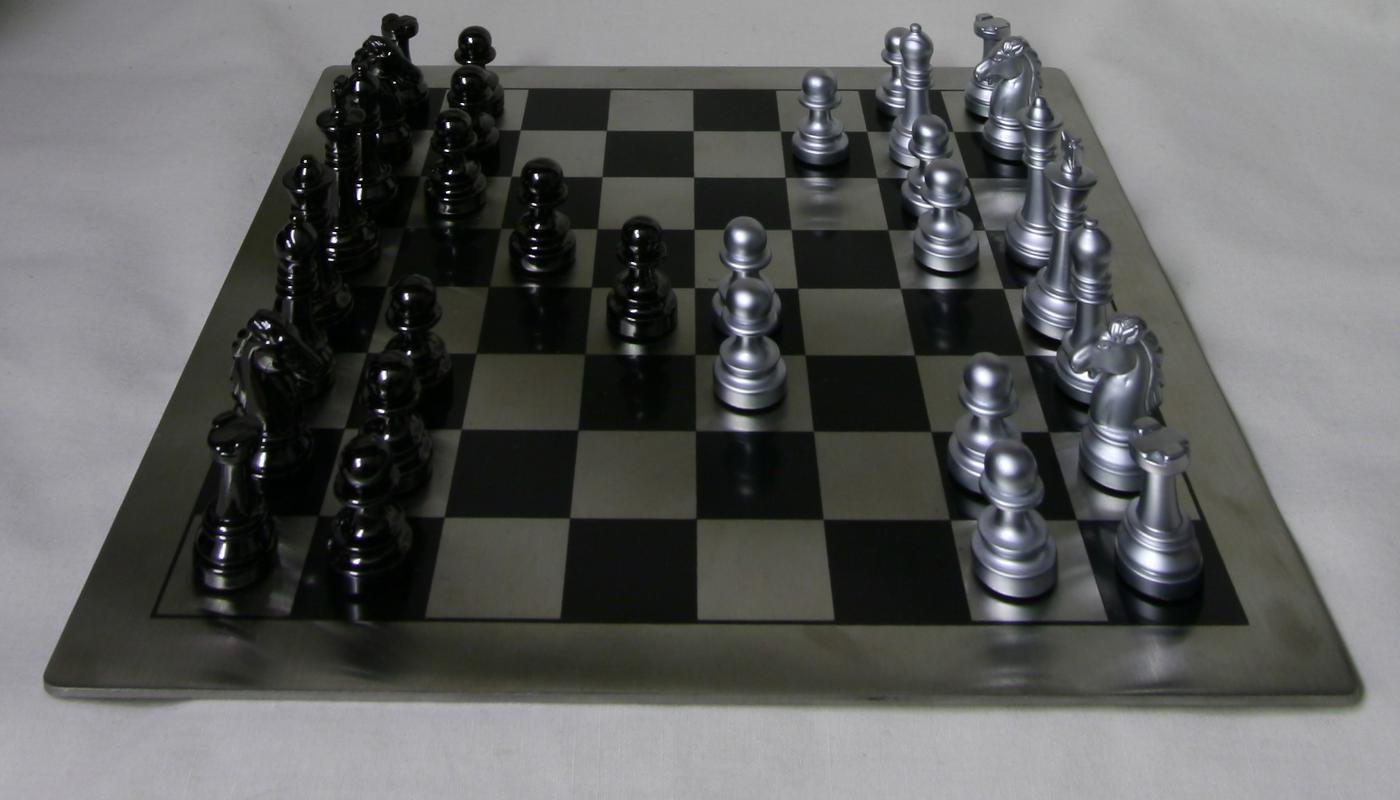
We used data from the Stanford Light Field Archive to demonstrate these effects. Each image was labeled with its corresponding (x,y) value in the 17x17 grid, as well as a (u,v) value that corresponded to its camera location offset. Thus, in total we were working with 289 subaperture images of the chessboard scene. Below are some sample images from this dataset. Through the sample images, we can see that while the scene is the same across images, the perspectives and the viewing angle is slightly different.

(x,y) = (8,4)

(u,v) = (-3314,-798)

(x,y) = (5,14)

(u,v) = (-3330,-848)

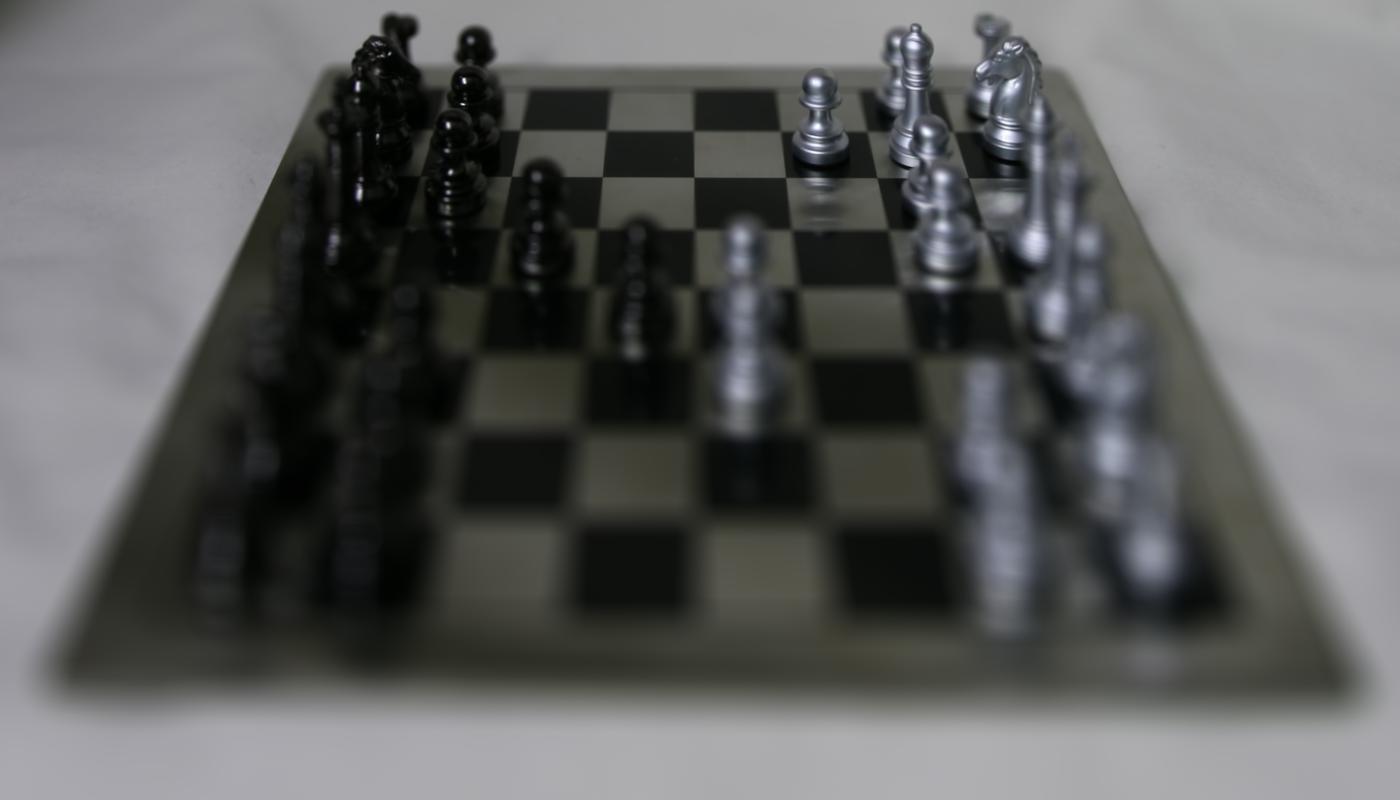
For thie first part of this project, we implemented refocusing at different depths. While the camera position varies over the subaperture images in the grid, the objects far away from the camera do not vary their position by much, while the objects closer to the camera shift their position much more greatly in comparison. By averaging all the subaperture images in the grid without any shifting, we end of producing an image of the scene that is sharp around the far objects and blurry around the near objects, as shown in the resulting refocused scene below.

To refocus the image around different depths of the scene, we implemented some shifting operations that took place before we averaged the images. The overall idea behind this was to align certain parts of the scene with each other across the various subaperture images before averaging, which would move the focus to the aligned area of the scene.

For each subaperture image at grid coordinate (x,y), we calculated its shift (s,t) with the following:

x_shift = c * (u_center - u)
y_shift = c * (v_center - v)

where (u,v) were the camera position coordinates corresponding to the subaperture image at (x,y) and (u_center, v_center) were the camera positions of the center grid image that we were aligning to. In this case (8,8) served as the center in our 17x17 grid. Finally, c was a constant that determined the amount of alignment that we would be shifting to. As we decreased c, the objects closer to the camera became sharper and as we increased it, objects further away became sharp.

For each subaperture image, we determined the appropriate shift amounts, and then proceeded to average all the shifted images in order to produce a refocused image. Below are a few refocused images with different values of c.

c = -0.55

c = -0.4

c = -0.25

c = -0.1

c = 0

c = 0.15

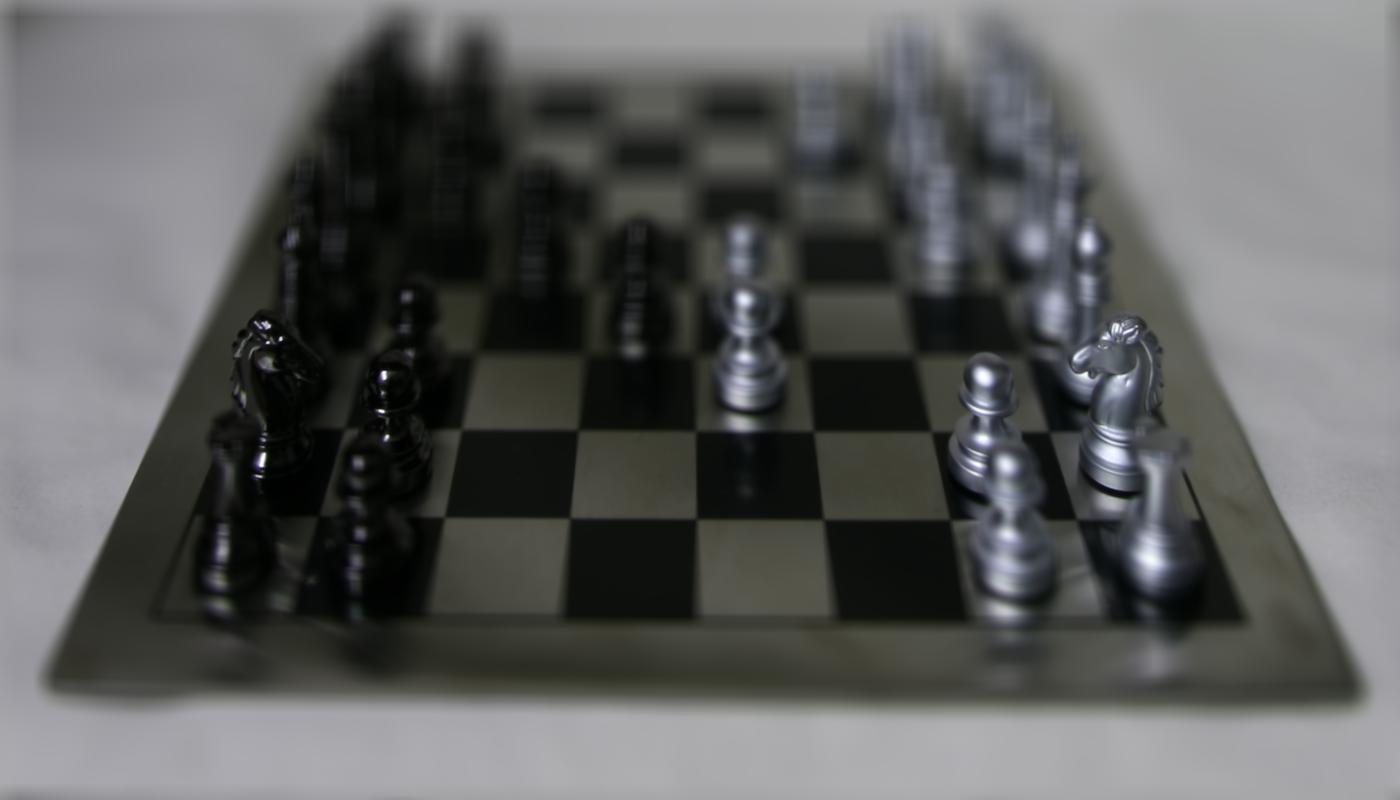
Here is a gif of my final results with c varying from -0.7 to 0.2. As the gif progresses, we can see the focus of the scene moving from the front, nearby objects to the back far objects.

Next, we also implemented aperture adjustment using the same lightfield data. Aperture is the size of the hole through which light enters the camera. Aperture has a direct effect on the depth of field. When the aperture is large, there is a smaller depth of field and as a result gives a shallow focus effect. Meanwhile, when the aperture is small, the depth of field is large, and a larger proportion of the image is in focus and sharp.

Averaging a large number of images sampled over the grid perpendicular to the optical axis mimics a camera with a larger aperture because when the images are sampled over a larger radius on the grid, there will be a larger blur effect when averaging the images together. Conversely, using fewer images results in an image that mimics a smaller aperture because when a smaller aperture is used, the hole throughout which light can enter is smaller and thus limits the amount of blurring that occurs in the image.

Using these concepts, we were able to apply an algorithm to produce scenes that mimic images with different aperture sizes. Using an input radius r, we kept images if their camera position was within r units away from the center grid image at (8,8). Then, we averaged across those images to produce the scene. We used the following equation to determine whether or not to keep an image for averaging:

sqrt ( (u - u_center)^2 + (v - v_center)^2 ) < r

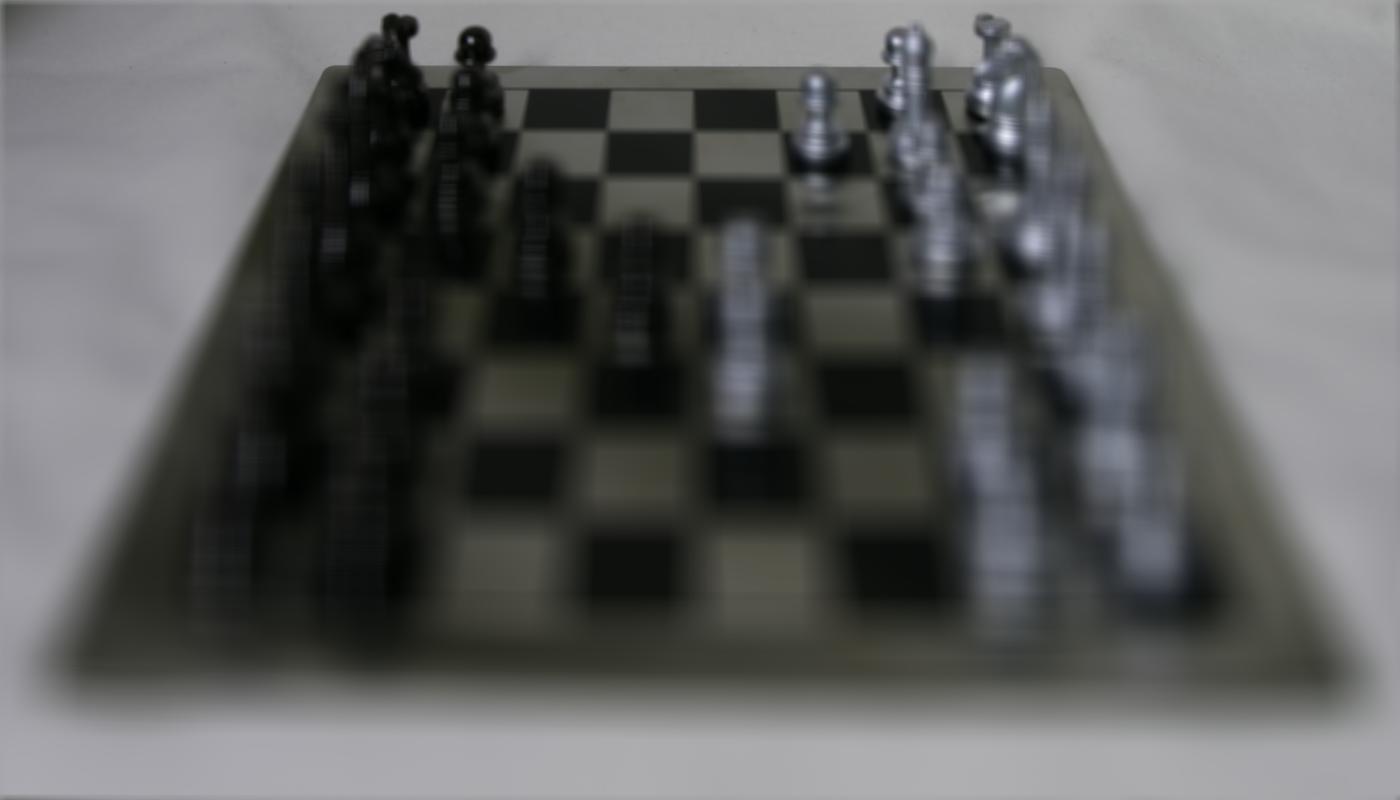
where (u,v) corresponded to the image's camera position, (u_center, v_center) corresponded to the center image's camera position, and r was the given radius. Below are some results of the aperture adjustment for different radius sizes.

r = 0

r = 15

r = 30

r = 45

r = 60

And finally, here is a gif with the radius increasing from 0 to 60. The aperture size starts out small, with most of the scene being very sharp, and then becomes progressively larger, as more of the scene becomes blurred.

Overall, I really enjoyed this project! It was interesting to be able to computationally play around with things like depth and aperture and to gain a better understand of how those work with regard to photography. I enjoyed learning about lightfield cameras and post-processing that can be used to create various effects on a scene. The lightfield images captures many directions of light that allow us to play around with these cool effects of depth refocusing and aperture adjustment.